Chapter 6 Functions

Functions are a very important feature of most/all programming languages. We have already seen and used a series of functions such as vector() and matrix() to create vectors and matrices, class() to retrieve the class, or head() and tail() to get the first/last few elements.

Instead of only using existing functions, we can write ourselves functions to do specific things for us. But why should we write functions? The most important reasons are:

DRY principle: Don’t repeat yourself. Functions let you reuse the same computational building block in different parts of a program or script.
Procedural programming: Procedural programming is a programming paradigm, a way to write well-structured (modular) code. Using functions allows one to add structure to the code which helps to increase readability and maintainability (find errors/bugs). The opposite would be to just write one line after another, an endless series of commands without a clear structure. Such code is also called spaghetti code and should be avoided whenever possible (always).
Testing/Debugging: When writing functions, one can split a larger project in separate smaller computational building blocks (a bit like Lego). One big advantage is that this allows us to test individual smaller blocks to ensure that they work properly. This makes it much easier to find potential bugs and errors (called debugging).

Writing functions is the key feature to evolve from a ‘basic user’ to a ‘developer’.

6.1 Functions in R

As everything else in R, functions are also first class objects (like vectors or matrices) and can be used in the same way. This allows one to pass functions as input arguments to other function which is frequently used and an important feature in R.

Example: To prove that we can work with functions like any other object in R, let us assign an existing function (min()) to a new object called my_minimum. This simply makes a copy of the function – the new object is, again, a valid function.

my_minimum <- min         # Copy the function
x <- c(10, -3, 20)        # Demo vector
my_minimum(x)             # Our function (copy)

## [1] -3

min(x)                    # Original function (returns the same)

## [1] -3

Functions consist of three key elements:

Input arguments (or parameters).
Instructions or code.
A return value (output).

All three are optional; some functions have no input arguments, others have no explicit return, and we can even write functions without instructions - which are absolutely useless, as they … just don’t do anything. Typically functions have at least input arguments and instructions, and most will also explicitly return a result, or at least an indication that the function successfully executed the instructions (we’ll come back to returns later).

Functions can also be nested (a function calls another function as part of the instructions) and can be called recursively (one function may call itself several times).

Functions are most often side effect free. That means that the functions do not change anything outside the function itself. They simply take over the input arguments as specified, go trough the instructions, and return the result back to the line where the function has been called. However, functions can have side effects. R uses something called “lexical scoping” which allows the function to access, delete, and modify objects which have not been explicitly used as argument to the function. This can be somewhat confusing and should be avoided (especially as a novice). We will come back to that at the end of this chapter.

When Should I Use Functions?

Avoid repetitions: Try to avoid copying & pasting chunks of code. Whenever you use copy & paste, it is a good indication that you should think about writing a function.
Facilitate reuse: Whenever similar code chunks should be used in different parts of the code, or even different scripts/projects.
Impose structure: Functions help you to structure your code and to avoid long and/or complex scripts.
Facilitate debugging: Allows for thorough quality control for important parts of the code (testing your function to ensure they work as expected).

Functions in real life

We all come across function-like situations in our daily life multiple times a day. One illustrative example are backing recipes. Imagine you are cooking some brownies:

Classical recipes are set up as follows:

A list of the required ingredients (the input arguments).
A set of instructions (mix this, do that, bake for 180 minutes)
And, last but not least, some (hopefully) tasty food! That’s the return value or output.

We can even find more analogies on this screenshot:

The name of the recipe is like the function name, the website where we have found the recipe is the name of the R package (if the function is included in a package).

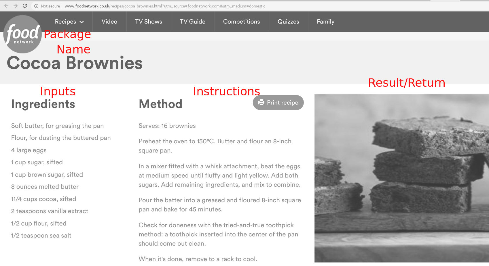
Every time we call this “function” (use this recipe) with this very specific name (Cocoa Brownies) from this specific package (or site, the food network) using the inputs (ingredients) as specified, we will always get the same result.

And that’s what functions do: perform specific tasks in a well-defined way, with a very specific return/result. And they can be reused over and over again, if needed.

6.2 Illustrative example

Before learning how to write custom functions, let’s motivate functions once again. Let us assume we have to calculate the standard deviation for a series of numeric vectors. As most likely well known from math, the standard deviation is defined as:

\(\text{sd}(x) = \sqrt{\frac{\sum_{i=1}^N (x_i - \bar{x})^2}{N - 1}}\)

Using a bit of math and some of the vector functions from the vectors chapter we can calculate the standard deviation of a vector x as follows:

# "Manually" calculate the standard deviation
sqrt(sum((x - mean(x))^2) / (length(x) - 1))

In words: take the square root (sqrt()) of the sum of \(x - \bar{x}\) (x - mean(x)) to the power of 2 (thus (x - mean(x))^2) divided by \(N - 1\) (length(x) - 1). Sure, there already is a function to calculate the standard deviation (sd()), but we will use our own code for this example.

We now have to calculate the standard deviation for three different vectors called x1, x2, and x3; e.g., for our thesis or as part of our job. For this example, the vectors just contain 1000 random values from the normal distribution.

What we do: We copy the code from above (for the standard deviation), insert it three times, adjust the names of the objects, and that’s it.

# Define the three vectors (random numbers)
set.seed(3) # Pseudo-randomization
x1 <- rnorm(1000, 0, 1.0)
x2 <- rnorm(1000, 0, 1.5)
x3 <- rnorm(1000, 0, 5.0)

# Calculate standard deviation once ...
sd1 <- sqrt(sum((x1 - mean(x1))^2) / (length(x1) - 1))
# ... and again, ...
sd2 <- sqrt(sum((x2 - mean(x2))^2) / (length(x2) - 1))
# ... and again ...
sd3 <- sqrt(sum((x3 - mean(x1))^2) / (length(x3) - 1))
c(sd1 = sd1, sd2 = sd2, sd3 = sd3)

##       sd1       sd2       sd3 
## 0.9980754 1.4957929 5.0425452

Even if the equation for the standard deviation is relatively simple you can already see that the code is quickly getting complex and prone to errors! Question: There is a bug in the code above! Have you noticed it? Solution hidden in the ‘practical exercise’ below.

Exercise 6.1 What have we done: We wrote the command for the equation of the standard deviation once for sd1:

sd1 <- sqrt(sum((x1 - mean(x1))^2) / (length(x1) - 1))

We tested this command and everything looked good. Thus, we copied the line twice for sd2 and sd3 and replaced x1 (as sd2 should be based on x2 and sd3 on the vector x3). However, we forgot to change one instance of x1 in the last line where we are calculating the standard deviation sd3 (should be x3 not x1 in the command on the right hand side).

#                        HERE
sd3 <- sqrt(sum((x3 - mean(x1))^2) / (length(x3) - 1))

This happens very easily and such bugs are often very hard to find, or will not be found at all (or after you published all your results, which may be all wrong due to such errors). Take home message: The copy & paste strategy is not a good option and should be avoided!

Rather than doing this spaghetti-style coding we now use functions. Below you can find a small function (we will talk about the individual elements in a minute; Declaring functions) which does the very same – it has one input parameter x, calculates the standard deviation (instructions), and returns it.

# User-defined standard deviation function
sdfun <- function(x) {
  res <- sqrt(sum((x - mean(x))^2) / (length(x) - 1))
  return(res)
}

Once we have the function, we can test if the function works as expected and then use it to do the same calculations again (as above). Note: If you would like to try it yourself we must execute the function definition above in the R console before we can use the function.

# Define some values
set.seed(3) # Pseudo-randomization
x1 <- rnorm(1000, 0, 1)
x2 <- rnorm(1000, 0, 1.5)
x3 <- rnorm(1000, 0, 5)

# Calculate standard deviation
sd1 <- sdfun(x1)
sd2 <- sdfun(x2)
sd3 <- sdfun(x3)
c(sd1 = sd1, sd2 = sd2, sd3 = sd3)

##       sd1       sd2       sd3 
## 0.9980754 1.4957929 5.0420466

I think you can see that this code chunk looks much cleaner and that we have avoided the mistake we made above. The code does not only look cleaner, it is much easier to read, easier to maintain, and (as we have tested our function) we know that the results are correct. An additional advantage: we can reuse the function again for other tasks or projects.

6.3 Calling functions

A function call consists of the name of the function and a (possibly empty) argument list in round brackets (function_name(...)).

We have already seen a series of such function calls in the previous chapters with and without input arguments such as:

getwd(): Return current working directory, a function call without arguments.
length(x): Returns the length of the object x (one unnamed argument).
matrix(data = NA, nrow = 3, ncol = 3): Create a \(3 \times 3\) matrix (multiple named arguments).

This is the same for all functions, even custom function written by ourselves. Note: in case you call a function which does not exist, R will throw an error and tells you that it could not find a function called like this. If so, check the name of the function you are calling (typo?).

some_function(x = 3)

## Error in some_function(x = 3): could not find function "some_function"

6.4 Naming functions

Functions can basically get any (valid) name. However, you may overwrite existing functions if the function name already exists.

Function names should be meaningful (don’t use f(), fun(), foo()).
They shoud be unique (don’t use mean(), sd(), print()), otherwise we might mask or overwrite existing functions.
Variable and functions with the very same name can co-exist (bad practice!).

An example of co-existence of a vector called mean and the function mean(). As both can exist at the same time, we can now calculate the mean() of the vector mean.

mean <- c(1, 2, 3, 4, 5, 6)  # Vector called 'mean'
mean(mean)                   # Function called 'mean()'

## [1] 3.5

Even if this works try to avoid such constructs as (even in this simple example) it is somehow confusing to understand what mean(mean) means :).

6.5 Declaring functions

Let us begin with an empty function. All parts of a function (input arguments, instructions, and output) are “optional”. If we don’t declare all three, that is what we will end up with:

myfun <- function() {
    # No instructions
}

Basic elements:

The keyword function(...) creates a new function.
(...) is used to specify the arguments (in the example above there are no arguments, thus () is empty).
Everything inside the curly brackets {...} is executed when calling the function (instructions; here empty/just a comment).
The new function() { } is assigned to a new object called myfun.

Inspect the object: As all objects in R we can also inspect our new object myfun.

class(myfun)          # Return class of the object

## [1] "function"

is.function(myfun)    # Check if the object is a function

## [1] TRUE

length(myfun)         # Length

## [1] 1

typeof(myfun)         # Type

## [1] "closure"

Functions are of class function, the type (closure) simply indicates a function.

Inspect the return value: Something which is a bit special in R: All functions have a return value. But haven’t we just learned that this is also optional? To be precise: explicit returns are optional. But even if we have no explicit return, a function in R always returns something. This return can be invisible and/or empty, indicated by the NULL value (empty object).

Our function myfun() has no explicit return value. Let us check if/what the function returns:

x <- myfun()
x

## NULL

… we get a NULL as the return value.

6.6 The `NULL` value in R

The NULL value in R is what the NoneType (‘None’) is in Python or ‘NONE’ in SQL to mention two examples outside R.

NULL is an empty object (NULL basically means ‘nothing’). However, as all objects in R NULL still has a class, a type, and a length. The length is obviously 0 (as the object is completely empty), while the class and type are both NULL. As for most other classes there is a function is.null() to check if an object is NULL.

x <- NULL
length(x)

## [1] 0

class(x)

## [1] "NULL"

typeof(x)

## [1] "NULL"

is.null(x)

## [1] TRUE

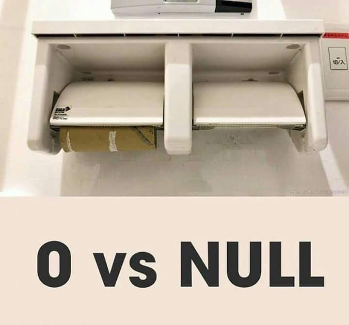
Figure 6.1: A quick geek joke: 0 versus NULL, source: http://i.imgur.com/7QMhUom.jpg

The message behind the image: We can still work with a numerical zero (e.g., \(0 + 10 - 5 = 5\)), while a NULL value cannot be used for anything useful, not even in an emergency situation as in the picture above.

6.7 Functions `cat()` and `paste()`

In the following sections we will use two new functions called cat() and paste(). Both have some similarities but are made for different purposes.

paste(): Allows to combine different elements into a character string, e.g., different words to build a long character string with a full sentence. Always returns a character vector.
cat(): Can also be used to combine different elements, but will immediately show the result on the console. Used to displays some information to us as users. Always returns NULL.

We will, for now, only use the basics of these two functions to create some nice output and will come back to paste() in an upcoming chapter to show what else it can do.

6.7.1 Concatenate and print

The function cat() is used to concatenate one or multiple elements and immediately show the result to us as users. Internally, all elements are converted to character and then put together, by default separated by a blank (a space) and then shown on the console.

This can be used to show a simple character string, combine multiple characters, or combine elements of different types to create easy-to-read output and information. Note: By default, cat() does not add a line break (or carriage return) at the end of what is shown. To get nice line-by-line output we can add a "\n" which is interpreted as a line break by our computer. A few examples:

# Output simple character string
cat("What a great day!\n")

## What a great day!

# Combine a variable `x` with a character string + \n
x <- "What a great day"
cat(x, "today!\n")

## What a great day today!

# Concatenate character strings and elements of named numeric vector
housecat <- c("height" = 46, "weight" = 4.5)
cat("The average house cat is", housecat["height"],
    "cm tall\nand weighs", housecat["weight"], "kilograms.\n")

## The average house cat is 46 cm tall
## and weighs 4.5 kilograms.

Note that cat() should not be confused with the function print(). print() is used to show the content of an entire object (e.g., a vector or matrix), while the purpose of cat() is to output some information for us.

And what does it return? The one and only purpose of cat() is to show information on the console, the function does solely return NULL (‘nothing’).

x <- cat("What does cat return?\n")

## What does cat return?

print(x)

## NULL

class(x)

## [1] "NULL"

6.7.2 Concatenate strings

The other function we will use is paste() which works similarly but is used for a different purpose. As cat(), paste() can take up a series of elements and combines them to a longer character string.

Instead of immediately showing the result on the console, this string will be returned such that we can store it on an object and use later. E.g., we can use the resulting string as a nice title for a plot. An example:

res <- paste("The average house cat is", housecat["height"],
             "cm tall\nand weighs", housecat["weight"], "kilograms.\n")

We create the very same character string as above, but now store the result on our new object res. Let us see what we have gotten:

length(res)

## [1] 1

class(res)

## [1] "character"

cat(res)

## The average house cat is 46 cm tall
## and weighs 4.5 kilograms.

paste() returned a character vector of length 1 with the combined information which we can use later on in our code, here simply forwarded to cat().

6.8 Basic functions

Let us start to write some more useful functions than the one in the section Declaring functions. Below you will find three functions (A - D) with increasing “complexity” to show the different parts of a function.

Function A

Name: say_hello.
Arguments: None.
Instructions: Outputs "Hello world!" on the console.
Return value: No explicit return (output).

say_hello <- function() {
    cat("Hello World!\n")    # Hello World + line break
}
# Call function
say_hello()

## Hello World!

As the function has no input arguments, nothing has to be declared between the round brackets (()) when calling the function. We are not even allowed to do so (try say_hello("test")).

Once called, the instructions are executed and "Hello world" will be shown to us. We have no explicit return, but as mentioned earlier all functions in R return something. What does this function return?

test <- say_hello()

## Hello World!

print(test)

## NULL

class(test)

## [1] "NULL"

By default R returns the ‘last thing returned inside the instructions’ which in this case is simply NULL from the cat() command. Not too important to understand, but keep this in mind.

In practice, we shall always define explicit returns in each and every function; we will come back to this in more detail later on.

Function B

Name: say_hello (same name; redeclare function).
Arguments: One argument x.
Instructions: Paste and output the result using cat().
Return value: No explicit return (output).

As shown in the instructions we have to adjust our function to have one input argument named x. We will use the content of x and combine it with "Good morning" to say hello to a specific person.

# Re-declare the function (overwrites the previous one!)
say_hello <- function(x) {
    cat("Good morning", x, "\n")
}
# Call function
say_hello("Jochen")

## Good morning Jochen

The difference to “Function A”: We now have one input argument to control the behaviour of the function. As there is no default (we’ll come back to that later) this is a mandatory argument. If we do not specify it, we will run into an error as the function expects that we do hand over this argument.

say_hello()

## Error in say_hello(): argument "x" is missing, with no default

Again, as we have no explicit return, the function will return the last thing returned internally, which is (again) the NULL value from cat(). However, in contrast to function A we now have a flexible function which can be used to say hello to anyone we like to.

say_hello("Helga")

## Good morning Helga

say_hello("Jose")

## Good morning Jose

Exercise 6.2 Non-character input

cat() can also handle data of other types, and vectors. Try and see what happens if you use an integer, a logical value, and a character vector as input argument (e.g., print_hello(123L)).

Use a single integer as input argument.
Use a logical value as input argument.
Specify a character vector (e.g., c("Francisca", "Max", "Sunshine")) as argument.

Solution. As you will see, the function still works – even if the result might be a bit strange ("Good morning TRUE"). The reason is that our input argument is simply forwarded to the paste() function, and the paste() function is able to handle all these cases without any problem.

(1) Integer as input

say_hello(1234L)

## Good morning 1234

(2) Logical value as input

say_hello(TRUE)

## Good morning TRUE

(3) Character vector as input

say_hello(c("Francisca", "Max", "Sunshine"))

## Good morning Francisca Max Sunshine

This function is not very specific. In reality, we might extend the function and check what is specified on the input argument x such that we can throw an error if the input is, e.g., not ‘a character vector of length 1’ (as we expect one name as input).

This is called a ‘sanity check’ (input check) which we will revisit at a later time.

Function C

Name: hello (new name).
Arguments: One argument x.
Instructions: Combine "Hi" and argument x and store the resulting character string on res. Do not print/show the result.
Return value: Explicit return of the result.

Let us declare a new function which we will call hello for now. This function no longer uses cat(), so it does not automatically show the result. Instead we are using paste() to create the welcome message, and then return that character to be used outside the function.

# Declare the function
hello <- function(x) {
    res <- paste("Hi", x)
    return(res)
}

The new function will now run completely silent (no information shown on console).

result <- hello("Peter")

Instead we get the resulting character string ("Hi Peter") returned by our function.

print(result)

## [1] "Hi Peter"

class(result)

## [1] "character"

Quick detour: `return()` and `invisible()`

Whenever writing a function, we shall always have an explicit return at the end of the function.

return(): Returns one object. The return value is printed unless assigned to an object (implicit printing).
invisible(): Also returns one object. Will not be printed, but can still be assigned to an object.

We declare two additional functions (hello_return and hello_invisible) to show the difference. Both functions do the same, except that one uses return() for the return value, the other one invisible() and use "Hi", and "Hello", respectively.

# Using return()
hello_return <- function(x) {
    res <- paste("Hi", x)
    return(res)
}

# Using invisible()
hello_invisible <- function(x) {
    res <- paste("Hello", x)
    invisible(res)
}

The difference can be seen when we call the two functions.

hello_return("Maria")

## [1] "Hi Maria"

hello_invisible("Maria")

When calling hello_return("Maria") we can immediately see the result ("Hi Maria"), while we do not get any output when calling hello_invisible("Maria") as the result is returned invisibly.

What if we directly assign the return of the two functions to two new objects?

result1 <- hello_return("Maria")
result2 <- hello_invisible("Maria")
print(result1)

## [1] "Hi Maria"

print(result2)

## [1] "Hello Maria"

Invisible returns are used frequently in R by a wide range of functions. One example is the function boxplot(). Typically, one is only interested in the figure, wherefore it is not necessary that boxplot() returns anything. However, there is an invisible return which contains the numeric values used to create the plot. An example using some random data:

set.seed(6020)         # Random seed
x   <- rnorm(200, 20, 3) # Draw 200 random values
res <- boxplot(x, main = "Demo Boxplot")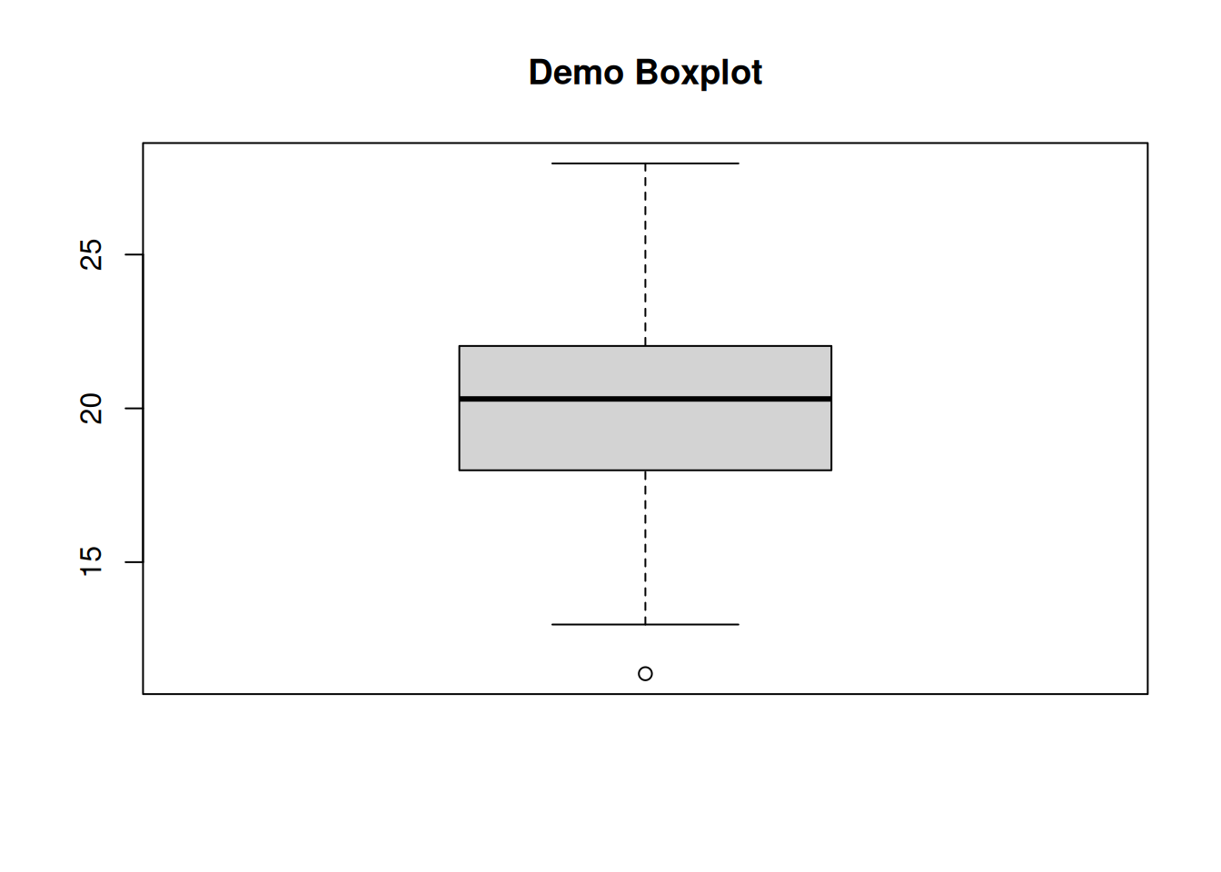

Let us check what the function returns (invisibly):

res

## $stats
##          [,1]
## [1,] 12.97141
## [2,] 17.98763
## [3,] 20.30682
## [4,] 22.02997
## [5,] 27.96467
## 
## $n
## [1] 200
## 
## $conf
##          [,1]
## [1,] 19.85520
## [2,] 20.75844
## 
## $out
## [1] 11.37251
## 
## $group
## [1] 1
## 
## $names
## [1] ""

The function returns a list with all the components used for plotting. E.g., stats contain the numeric values for the box-and-whiskers, n the number of values used for the plot, and out the outliers (plotted as a circle).

Function D

So far, our functions always returned a character string. A function can, of course also print one thing, and return something else. Let us create one last function in this section.

Name: hello (redeclare the function).
Arguments: One argument x.
Instructions: Use paste() to create the character string and show it on the console using cat(). Then, calculate (count) the number of characters in this string.
Return value: Explicit return; number of characters of the newly created string.

# Re-declare the function
hello <- function(x) {
    # First, create the new string using paste, and immediately print it
    # As we no longer need 'x' later on, we simply overwrite it here.
    x <- paste("Hello", x)
    cat(x, "\n")
    # Count the number of characters in 'x'
    res <- nchar(x)
    # Return the object 'res'
    return(res)
}

When calling the function we now expect that the character string is printed, and that the function returns the number of characters (letters) in this string. Let us try:

result <- hello("Max")

## Hello Max

When calling the function, we can immediately see "Hello Max". This is caused by calling cat() inside the function. But let us see what the function returned.

class(result)

## [1] "integer"

result

## [1] 9

What we get in return is an integer vector which contains 9. This is the number of characters in "Hello Max" ("Hello" has five characters, "Max" another three, plus \(1\) for the space in between, thus 9).

6.9 Alternative syntax

In R, things can sometimes be written in slightly different ways, which also yields for function definitions. Below you can find a series of definitions for a simple function add2 which returns x + 2; all definitions do the very same.

Brackets and explicit returns (version 1) are typically preferred. For very short functions as this one, one-liner versions can also be OK.

Version 1: The preferred one.

add2 <- function(x) {
    return(x + 2)
}

Version 2: One-liner.

add2 <- function(x) { return(x + 2) }

Version 3: Without brackets.

add2 <- function(x) return(x + 2)

Version 4: Without brackets, without explicit return.

add2 <- function(x) x + 2

Version 5: Without explicit return (but brackets).

add2 <- function(x) {
    x + 2
}

6.10 Arguments

Multiple arguments

So far, our function(s) always only had one single input argument. More often than not, functions come with multiple arguments.

Let us extend the function from above (the hello function) and add a second argument which will be called greeting. The first argument (main input) is often called x or object, we will stick to x here.

# Re-declare the function once more
# Shows the message using cat() and invisible returns the same
# character string to be used later if needed.
hello <- function(x, greeting) {
    res <- paste(greeting, x)
    cat(res, "\n")
    invisible(res)
}

Both arguments are required arguments. When calling the function, we must specify both. As in the function declaration, the arguments are separated by a comma (,).

hello("Jordan", "Hi")

## Hi Jordan

hello("Reto", "Good afternoon")

## Good afternoon Reto

Remark: Why this strange order of input arguments? Wouldn’t it be logical to put the input greeting before x? Well, we could also change the order and define the function as follows (new function hello2):

# Declare a second 'hello2' function
hello2 <- function(x, name) {
    res <- paste(x, name)
    cat(res, "\n")
    invisible(res)
}
# Calling 'hello2()' and 'hello()'
hello2("Hi", "Eva!")

## Hi Eva!

hello("Eva!", "Hi")

## Hi Eva!

As you can see, both functions do the very same, except that the input arguments are flipped. We will come back to this example when talking about default arguments where we will see that the ‘reverse order’ of the arguments can make sense when combined with defaults.

Missing arguments

What if we forget to properly specify all required arguments? In this case R throws an error and tells us which one was missing (here greetings). Again, R is very precise to tell us what has been going wrong – try to get used to properly read error messages.

hello("Rob")

## Error in hello("Rob"): argument "greeting" is missing, with no default

But: This only causes an error if the argument is evaluated in the function. If not used at all, no error will be thrown.

# Additional (unused!) argument 'prefix'
hello <- function(x, greeting, prefix) {
    # Combine and return
    res <- paste(greeting, x)
    cat(res, "\n")
    invisible(res)
}
hello("Rob", "Hello")

## Hello Rob

In this case the additional argument prefix is never used in the instructions. In such a situation there will be no error. This is, however, a very bad example to follow – if there are input arguments they should also be used in some way.

Argument specification

When calling functions, the arguments to the function can be named or unnamed. Named arguments are always matched first, the remaining ones are matched by position.

Let us use this function again:

# Re-declare the function
hello <- function(x, greeting) {
    res <- paste(greeting, x)
    cat(res, "\n")
    invisible(res)
}

All unnamed: When calling the function with two unnamed input arguments, the arguments are used in this order (the first one will be x, the second one greeting).

hello("Rob", "Hello")

## Hello Rob

All named: Alternatively, we can always name all arguments. In case we name both, the order does not matter as R knows which one is which one.

hello(x = "Rob", greeting = "Hello")

## Hello Rob

hello(greeting = "Hello", x = "Rob")

## Hello Rob

Mixed: If we mix named and unnamed arguments, the named ones are matched first. The rest (unnamed arguments) are used for the remaining function arguments in the same order as we provide them.

hello(greeting = "Hello", "Rob")

## Hello Rob

First, the named one (greeting) is matched. The second (unnamed) argument "Rob" is then used for the remaining input arguments we have not explicitly defined. All left is our input x, thus "Rob" is used as x. The same happens for these three function calls (try it yourself):

hello("Rob", greeting = "Hello")

## Hello Rob

hello(x = "Rob", "Hello")

## Hello Rob

hello("Hello", x = "Rob")

## Hello Rob

In practice: Often the first (main) arguments are unnamed and defined by its position, the others by name.

hello("Rob", greeting = "Hello")

## Hello Rob

Partial matching

Partial matching is used if the argument names are incomplete. As an example:

hello("Rob", gr = "Welcome")

## Welcome Rob

This works as long as gr only matches one of the arguments (greetings). One classical example where people often use it is the sequence function (seq()) we have seen in the vectors chapter (Numeric sequences). The documentation (?seq) function has an argument length.out:

length.out: desired length of the sequence.  A non-negative number,
          which for ‘seq’ and ‘seq.int’ will be rounded up if
          fractional.

However, you will frequently see that people only use length and rely on the partial matching used by R.

seq(0, 5, length = 4)

## [1] 0.000000 1.666667 3.333333 5.000000

In practice: Try to avoid partial matching in programming tasks and use the full name of the arguments.

Partial matching: Taken to the extreme.

The function we will use returns a sequence. The two arguments are the start of the sequence, and the step width.

# Declare the function
step_fun <- function(start, step.width) {
    return(seq(start, by = step.width, length.out = 5))
}

Let us start with using full argument names, and continuously reduce the names to see how far we can go.

step_fun(start = 0, step.width = 0.2)

## [1] 0.0 0.2 0.4 0.6 0.8

step_fun(start = 0, step       = 0.2)

## [1] 0.0 0.2 0.4 0.6 0.8

step_fun(sta   = 0, ste        = 0.2)

## [1] 0.0 0.2 0.4 0.6 0.8

step_fun(st    = 0, st         = 0.2)

## Error in step_fun(st = 0, st = 0.2): formal argument "start" matched by multiple actual arguments

In the last example it is no longer possible to match the two arguments – thus we get an error. Again: Try to avoid partial matching in real life!

Default arguments

Another important feature of functions is the ‘default arguments’. A default argument definition allows one to define ‘optional’ arguments. The user can always specify them if needed, if not explicitly specified in the function call, the default value will be used.

Let us come back to the function hello() used in the section Multiple arguments.

hello <- function(x, greeting) {
    res <- paste(greeting, x)
    cat(res, "\n")
    invisible(res)
}

It was mentioned that the order of the two arguments look a bit weird. However, if we work with default arguments the order of the two input arguments might make sense. Let us redeclare the function:

Name: hello (redeclare function).
Arguments: Two arguments.
1. x: First (main) argument, mandatory (no default).
2. greeting = "Hello": Second argument, by default "Hello" will be used.
Instructions: Combine greeting and x using paste() and show the result using cat().
Return value: Invisible return the result of paste().

# Re-declare the function
hello <- function(x, greeting = "Hello") {
    res <- paste(greeting, x)
    cat(res, "\n")
    invisible(res)
}

The default makes the second argument an optional argument. This is often used for arguments that have a standard specification rarely to be changed, or used for ‘fine-tuning’.

hello("Rob")

## Hello Rob

hello("Isa", "Welcome to the lecture")

## Welcome to the lecture Isa

This allows us to change the default behaviour if needed, but don’t require to specify it when we use the function in a ‘default’ way.

We already came across functions with default arguments in the previous chapters. The default values are also always shown in the manual of the corresponding functions (check out ?seq, ?matrix).

seq(): By default from = 1, to = 1, by = 1.
matrix(): By default data = NA, nrow = 1, ncol = 1.

Lexical scoping

One more thing we should be aware of is lexical scoping. To clarify the jargon:

Name binding: Association of a variable with a certain value.
Scope: Part of a program where a certain name binding is valid.

In R:

Variables are typically created inside a script or inside the function where they are also used.
However, “free” variables may also be taken from the environment in which the function was defined (the function “grabs” an object from outside the function itself).
Can be useful, but also very confusing.
Advice: Try to avoid lexical scoping, especially in the early days of your programming career.

An example to demonstrate scoping: The following function takes one input argument x and returns x^power (\(x^\text{power}\)).

powfun <- function(x) {
    res <- x^power
    return(res)
}
powfun(2)

## [1] 4

powfun(3)

## [1] 9

Seems we get \(2^2\) and \(3^2\), but what is actually happening here? Well, the variable power <- 2 was defined in the same environment, but not shown in the book.

This happens:

We call the function with some specific argument for x.
The instructions of the function will be evaluated.
- The function wants to calculate x^power.
- power is not defined inside the function, thus R (the function) tries to find an object called power outside the function.
- If such an object exists, it will be used for the calculation (or else we will get an error).
The result is returned as expected.

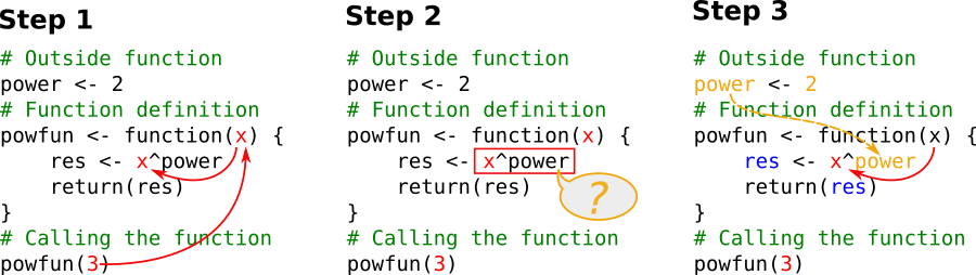
Figure 6.2: Simple example of lexical scoping.

Clear by now: Another example to illustrate a simple function which makes use of scoping is the following:

x <- "the one from the outside"
printx <- function() {
    res <- paste("x is", x)
    cat(res, "\n")
    invisible(res)
}
printx()

## x is the one from the outside

But: Nested lexical-scoped functions make affairs even more complex.

nestfun <- function() {
    x <- "the one from the inside"
    printx2 <- function() {
        res <- paste("x is", x)
        cat(res)
        invisible(res)
    }
    printx()
    printx2()
}
nestfun()

## x is the one from the outside 
## x is the one from the inside

6.11 Summary

The following should be kept in mind when working with functions:

Use functions to not repeat yourself (DRY principle), to structure your code, and to test specific parts of your program.
Use meaningful function names, don’t overwrite existing functions.
Variables to be defined by the user should be proper arguments; remove unused arguments.
Make use of default arguments for inputs used to ‘fine-tune’ function calls.
Declare all variables inside the corresponding function, avoid free variables and scoping unless it is useful for a certain task and you know what you are doing. Not recommended for novices.

6.12 Basic workflow

Especially for beginners, writing functions (compared to standalone code) can be a bit difficult. One way to get used to write functions is to do this in steps. After a while you may not need this step-by-step workflow anymore.

Let us use the data set `persons.rda` (click for download) for demonstration.

First steps for beginners

Start with a fresh script (.R).
Step 1: Develop standalone code (without new functions).
Step 2: When everything works, wrap (block of) code into a function.
Step 3: Refine/adjust/extend the function.
Afterwards, test your function. Does it work as expected?

Step 1: We would like to create a new function find_tallest_man() with one input argument called persons, the object stored in `persons.rda`. The steps we need to perform are:

Load the data set and investigate the object.
Find all rows containing males (where gender == 0).
Find the tallest man.

# Clear workspace
rm(list = objects())
# Load object, check what we got
load("persons.rda", verbose = TRUE)

## Loading objects:
##   persons

head(persons)

##         height   age gender
## Renate     155 33.07      1
## Kurt       175 22.36      0
## Hermann    171 18.68      0
## Anja       152 18.96      1
## Andrea     165 45.52      1
## Bertha     155 24.40      1

class(persons)

## [1] "matrix" "array"

# Find rows containing male persons (logical vector)
idx <- persons[, "gender"] == 0
# Extract heights of all male persons
heights <- persons[idx, "height"]
# And find the tallest person (one way to do so)
tail(sort(heights), n = 1)

## Uwe 
## 194

Step 2: Once this works, we can adjust our .R script and put the necessary instructions into a new custom function. Note: the first few lines (clear workspace, load/investigate data set) are not part of the function.

# Clear workspace
rm(list = objects())
# Load object, check what we got
load("persons.rda")

# Start with our new function
# Name:       find_tallest_man
# Arguments:  persons, matrix, data set.
# Return:     Return tallest male person.
find_tallest_man <- function(persons) {
    # Find rows containing male persons (logical vector)
    idx <- persons[, "gender"] == 0

    # Extract heights of all male persons
    heights <- persons[idx, "height"]

    # And find the tallest person, return result
    result <- tail(sort(heights), n = 1)
    return(result)
}

# Test out function
find_tallest_man(persons)

## Uwe 
## 194

So far, so good. Important: check that all objects used inside the function are properly defined, either as arguments to the function or defined inside the function (avoid scoping).

Step 3: Refinements and extensions. We can now adjust and extend the function. In this example we are doing the following:

Name: Rename the function to find_tallest_person().
Arguments:
- Rename first argument (main argument) to x. Take care: if we do this, we need to replace all occurences of the variable inside the function!!
- Add second argument n = 1 (number of tallest persons we would like to get, default 1).
- Add third argument gender = c(0, 1). Gender of the tallest persons, by default 0 or 1 (male and female).
Instructions: Similar to what we have had before, additional sanity checks at the beginning (Note: we will come back to sanity checks in more detail in the next chapter).
Return: Same object as before.

# Clear workspace
rm(list = objects())
# Load object, check what we got
load("persons.rda")

# Start with our new function
# Name:       find_tallest_person
# Arguments:  persons, matrix, data set.
# Return:     Return tallest male person.
find_tallest_person <- function(x, n = 1, gender = c(0, 1)) {
    # ----------- sanity check -------------------------------
    stopifnot(is.matrix(x))                                  # Input 'x' must be a matrix.
    stopifnot(all(c("gender", "height") %in% colnames(x)))   # Must contain 'gender' and 'height' (column names)
    stopifnot(is.numeric(n), n > 0)                          # Input 'n' must be positive numeric
    stopifnot(is.numeric(gender))                            # Gender must be numeric

    # ----------- main part of the instructions --------------
    # Find rows in 'x' matching the gender we are looking for
    idx <- x[, "gender"] %in% gender

    # Extract corresponding 'height's from matrix 'x'
    heights <- x[idx, "height"]

    # And find the tallest person, return result
    result <- tail(sort(heights), n = n)
    return(result)
}

We can now test our function again. By default it should return one person (n = 1), can either be male or female (gender = c(0, 1)).

# Default call
find_tallest_person(persons)

## Uwe 
## 194

However, due to the refinement we can now also use the function to find the two tallest females in the data set …

find_tallest_person(persons, n = 2, gender = 1)

##     Julia Elisabeth 
##       167       169

… or the three tallest males.

find_tallest_person(persons, n = 3, gender = 0)

## Frank  Hans   Uwe 
##   188   189   194

Important: Double-check that the function (instructions) does no longer use persons as we renamed the argument to x. Check that the additional arguments are properly specified and used inside the function (e.g., head(..., n = n)).