Chapter 1 Introduction
This chapter gives a brief introduction to programming in general (what is programming, and why should we know how to program?) before introducing the R programming language and its history.
1.1 Programming
Programming is the way of telling a computer how to do certain things by giving it (unambiguous) instructions. The person who writes these instructions (you) is called a programmer, the instructions itself are called a program. Instructions can be written in many different ways, depending on the task which has to be done. The format in which instructions are written are called programming languages.
Why should I learn to code? Nowadays, tech is everywhere: in laptops and smartphones, the display panel at the bus stop, the automatic doors at this university, and even in your coffee machine. Learning to code improves your problem-solving and logical skills and teaches you how to efficiently solve a specific problem. You’ll quickly see that there is a solution for everything and being able to write small or large programs will make things (much!) easier. Spending less time on solving a complex and/or repetitive problem gives you more time to learn new things, think outside the box, and to develop new and interesting (research) questions.
Furthermore, being able to code will also increase your chances on the job market. Understanding what programs can do and how they can be deployed is more and more required in companies of all sizes and sectors. Even if you might not be employed as a full-time programmer; having a programming background helps you to improve communication, e.g., between you and your colleagues, customers, or teammates.
And, last but not least, programming is so much fun! Writing programs can be extremely creative, if one allows it to be.
1.2 Why not natural languages?
Natural languages, such as German or English, are (i) ambiguous (the same sentence/words in different situations may have different meanings), are (ii) fuzzily structured (we all know that there are always exceptions to the basic grammar rules), and (iii) have large (changing) vocabularies. For a computer, understanding natural languages is extremely difficult.
Examples:
- I got struck by a bolt. (A bolt can be a small piece of metal, or lightning. One hurts, the other one is quite likely life threatening).
- Ich sollte den Baum umfahren. (In German “umfahren” can be “drive around the obstacle” or “run it down”/“run over it”)
Thus different explicit languages have been developed for different tasks.
Mathematicians designed a very strict mathematical notation (e.g., 10 + 1 = 11, 100 / 5000 = 0.2). Another example are chemists who use a very strict
notation for chemical equations (e.g., \(CH_4 + 2\,O_2 \rightarrow CO_2 + 2\,H_2O\)). Very similar, computer scientists had to define a language which
allows them to give a machine some instructions such that it does what it
should do. This is what we call a programming language. As computers are “stupid”
(they have no common sense) programming languages have to have relatively few
and exactly defined rules and strictly controlled vocabularies. Every word (can
be a variable name, a function, or a command) has to be defined before it can
be used and can only be defined once (at a time).
1.3 History of programming
Modern programming goes back to the first part of the last century. The Z1, developed by Konrad Zuse (Germany) is known as the first modern programmable binary calculator. The Z1 was still a mechanical machine and, unfortunately, very complex and unreliable. Modern electronic computers were developed during/after the second world war. Back in these early years programs were often stored on so called punched cards (pieces of cardboard/paper with holes). The first high-level programming language was Fortran developed back in 1954 - and still in use. Some more facts:
- 1938: Z1 by Konrad Zuse (GER)
- 1945: first operational modern computer (U.S.)
- 1950: first computer where the program was stored in memory
- 1954: first high-level programming language (Fortran)
- 1974: Xerox Alto, first workstation
- 1976: IBM 5100, first laptop (weight: 25 kg; display size: 5’’)
- 2000+: first smartphones
Since then (starting with Fortran in 1954) a wide range of programming languages have become available. An up-to-date list of programming languages can be found here.
.](images/01/01_history_of_programming_languages.jpg)
Figure 1.1: History of programming languages, Source: visualinformation.info.
1.4 Number of languages
Today, 7117 different living natural languages are known (recognized by ISO 639) and 8945 programming languages (including different versions of the same software; see hopl.info).
If programming languages are explicit and well defined, why do we need so many different ones? Well, depending on the task, different languages have different advantages and drawbacks. Some programming languages have been designed for web applications, others for mobile devices, to solve mathematical systems fast and efficient, or to provide tools for data analysis. Some have their focus on being platform independent (run on different operating systems), others to be used for parallel computing. A “one for all” programming language does not exist and will quite likely never exist in the future.
For those interested:
1.5 The R programming language
What is R?
R is a programming language and free software environment for statistical computing and graphics maintained and supported by the R Foundation for Statistical Computing. And, of course, R also has its own history. The software we use today originates from S developed by John Chambers back in 1976 and was originally written to make his own life easier while working at the Bell Labs (a personal toolbox for internal data analysis). The software was originally written as a set of Fortran libraries but has been rewritten in C in 1988. S was exclusively licensed (and eventually sold in 2004) to a company that developed a commercial statistics system S-PLUS with graphical user interface on top of S.
In 1991 Ross Ihaka and Robert Gentleman at the Department of Statistics, University of Auckland, started working on a project that will ultimately become R. Officially, R first got announced in 1993 (32 years ago), was published as open-source software under the GPL (General Public License) in 1995, and finally R 1.0.0 was released on 2000-02-29, implementing the so-called S3 standard. The current version (version 4.3.1) has been released in June 2023, and is updated regularly (see r-project.org).
- 1976: John Chambers and co-workers at Bell Labs start working on S (S1, Fortran).
- 1988: S rewritten in C, first version of S-PLUS.
- 1993: S3 including object orientation and comprehensive statistical modeling toolbox.
- 2004: S sold to company developing S-PLUS (now Tibco).
- 1991: R development started by Ross Ihaka and Robert Gentleman.
- 1993: R first official release.
- 1997: R Core Team and Comprehensive R Archive Network (CRAN) established.
- 2000: R 1.0.0 released (implementing S3).
- Current release: R version 4.3.1. (check news on r-project.org)
Why is it important to know the history of R? Well, first of all because a lot of people will ask you why R is called R (for sure). And secondly because it is important to keep in mind that R (also S and S-PLUS) is written by statisticians for statisticians (in a broad sense). This is the biggest advantage of R but has also led to some quirks or peculiarities that are different from other major programming languages developed by computer scientists.
One important aspect of R is that R is free! It’s free as in free speech, not only as in free beer, and released under the GNU Public License (GPL) which guarantees four essential freedoms:
- Freedom 0: The freedom to run the program as you wish, for any purpose.
- Freedom 1: The freedom to study how the program works, and change it so it does your computing as you wish. Access to the source code is a precondition for this.
- Freedom 2: The freedom to redistribute copies so you can help others.
- Freedom 3: The freedom to distribute copies of your modified versions to others. By doing this you can give the whole community a chance to benefit from your changes. Access to the source code is a precondition for this.
Open science
Open-source software is an essential part of good open science practice and help to make research transparent and reproducible. The backbone of good open science:
- Open data.
- Open-source software/code.
- Open methodology.
- Open peer review.
- Open-access publication.
Furthermore, open-source software (open science in general) allows to learn and benefit from others, improve existing methods, and support others.
R on the job market
R is one of the leading programming languages for data science on the job market. The figure below shows the frequency which different programming languages have been mentioned in job announcements for open data science positions.
.](images/01/01_fossbytes_com.png)
Figure 1.2: Source: fossbytes.com.
1.6 The R ecosystem
As other programming languages (Perl, Python, …) the R system is modular. The base installation only provides a ‘small’ set of features (base/recommended packages) but can easily be extended by installing additional packages.
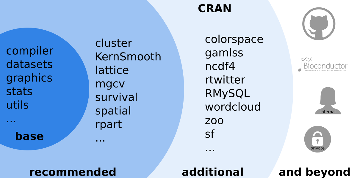
Figure 1.3: Overview over the large R ecosystem.
The main source for contributed packages is the Comprehensive R Archive Network (CRAN). However, other sources exist such as (Bioconductor) (R tools for bioinformatics, https://www.bioconductor.org/), private and community projects on https://GitHub.com/, or private packages. Packages exist for nearly everything and different packages may provide similar features, however, not all packages do have the same quality or are carefully maintained. Thus, it is recommended to use packages published via CRAN (or Bioconductor) as they undergo some quality control and automated checks while some private packages (e.g., from GitHub) may not work on all operating systems or R versions.
Another important aspect of all programming languages is to communicate with the outside world to import and export data (see also R Data Import/Export manual) or to communicate over a network.
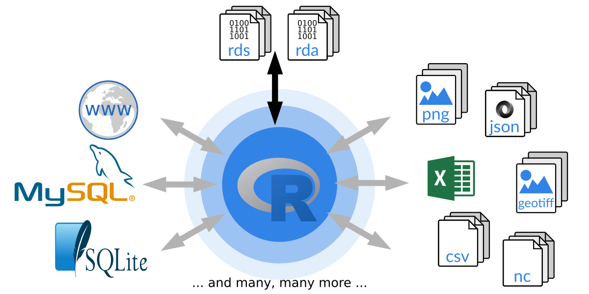
Figure 1.4: How R can communicate with the outside world.
R comes with a custom binary file format. These binary files are typically
called .rda/.rds (or sometimes .Rda/.RData or .Rds, respectively) and are used to store/load R objects.
Beside its own format R allows to read and write data from and to (nearly)
all available file formats. R base provides some high-level functions to
easily import data from human readable files (e.g., csv or ASCII in
general) which is often used for simple data sets. However, there is
basically no limit to read and write data in R and packages exist for nearly
all file formats, e.g., XLS/XLSX, XML, JSON, NetCDF, rastered data
sets such as geotiff, images in general (png/jpg/gif), databases
(sqlite/SQL) and many many more. If no package exists, feel free to
develop one yourself and contribute it to the R community! R also provides
socket connections for server-to-server connections over the network.
1.7 Examples
Now that we know what R is, what can we do with it? Well, basically everything you can think of! Your own creativity is the limit - and your programming skills, but we’ll work on that. In this course we will start with basic programming in R to get used to the language, data types and objects, and main control features and functions. The more complex the task, the more complex the program, but the fundamentals won’t change. Thus it is very important to acquire solid knowledge of the basics before proceeding to more complex tasks.
The concepts are not R specific and can easily be transfered to other programming languages; the language (names of functions and commands) is R specific, but modern programming languages are often very similar and once you’ve learned R starting with another programming language should not be a major hurdle.
Empirical mean and quartiles
A simple example of a program (one function) to calculate the empirical mean
and the 1st and 3rd empirical quartile of a set of 1000 random numbers from
a standard uniform distribution
using runif(). runif() returns one (or several) random numbers from the
uniform distribution, by default between \(0\) and \(1\):
## [1] 0.6639324## [1] 0.005586625Side note: As the distribution is symmetric, the mean is asymptotically
identical to the median (or the 2nd quartile). Theoretically the thee quartiles
should be 0.25, 0.50, and 0.75. Let’s try and draw 1000 random
numbers, store them on variable x. x will thus become a numeric vector of
length 1000. With head(x) we can show the first few (by default: six) observations
from x.
## [1] 0.8650577 0.6750063 0.4412765 0.9875925 0.9241197 0.9757181The second is to create a function which does the job for us. We create a
function called fun() which requires one input argument x and calculates the
empirical mean (m), the 1st quartile (q1) and the 3rd quartile (q3).
At the end a numeric vector of length 3 will be returned containing all three
values (c(q1, m, q3)), rounded to three digits by default. Once our function fun() is
defined we can call it using our random numbers as input (fun(x)) to get the
result. Et voila.
fun <- function(x, digits = 3) {
    m  <- sum(x) / length(x)
    q1 <- sort(x)[round(length(x) * 0.25)]
    q3 <- sort(x)[round(length(x) * 0.75)]
    return(round(c(q1, m, q3), digits))
}
fun(x)
## [1] 0.233 0.497 0.773We can, of course, use this function over and over again. Let’s draw another 1000 values from the uniform distribution and call the function again:
## [1] 0.237 0.493 0.736Of course R provides built-in functions to compute these quantities. One could e.g., use the
summary() method or the mean() and quantile() functions. Let’s have a look if our
function works as intended:
## [1] 0.2333466 0.4969940 0.7732961## 25% 75%
## 0.2333466 0.4969940 0.7732961## Min. 1st Qu. Median Mean 3rd Qu. Max.
## 0.0001134 0.2334573 0.4899650 0.4969940 0.7733465 0.9993777Notes: The summary method uses slightly different version of empirical quantiles. Also, as random data are used you will never get the same results (unless you initialize the random number generator using a so-caled random seed).
Statistical modeling
One of the biggest strengths of R is, of course, the wide range of functions and methods for data analysis and statistical modeling from simple linear regression models to more complex and flexible techniques.
This is just a very small example of a simple and basic workflow.
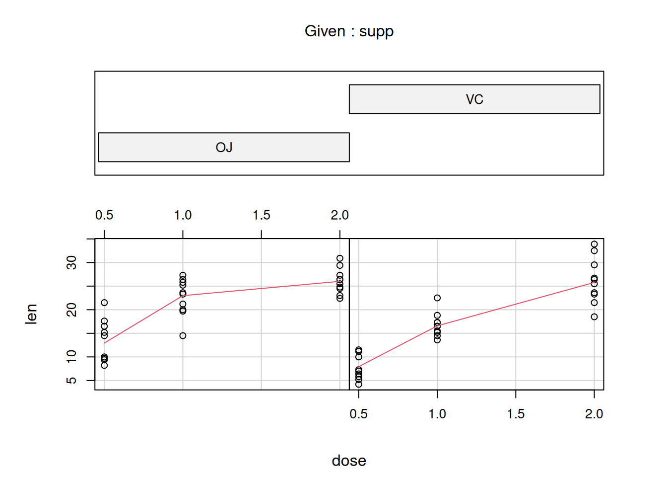
We are using a data set which is contained in datasets package (comes with
R base) called ToothGrowth (see ?ToothGrowth for details).
The data set contains observations of the length of a special cell which is
responsible for the growth of the teeth in 60 guinea pigs (whose teeth grow
for the entire life). The experiment investigates the impact of vitamin C on
the tooth growth. One group received orange juice
(OJ), the other one ascorbic acid (a form of vitamin C; VC). Each
individuum got either 0.5, 1.0, or 2.0 milligrams per day.
Variables:
len: numeric, tooth length.supp: factor, supplement type (VCorOJ).dose: numeric, dose in milligrams per day.
The data set (or data.frame in R) can be explored by looking at the first few rows (default: six)
using head(), computing a short summary() for each variable, or by
visualizing the data with a coplot() of length vs. dose grouped by supplement.
##    len supp dose
## 1  4.2   VC  0.5
## 2 11.5   VC  0.5
## 3 7.3 VC 0.5## len supp dose
## Min. : 4.20 OJ:30 Min. :0.500
## 1st Qu.:13.07 VC:30 1st Qu.:0.500
## Median :19.25 Median :1.000
## Mean :18.81 Mean :1.167
## 3rd Qu.:25.27 3rd Qu.:2.000
## Max. :33.90 Max. :2.000The two supp groups are plotted separately with the orange juice group on the
left-hand side and the ascorbic acid group on the right-hand side.
Estimate a linear model on the ToothGrowth data set. Length (len) of the
cells responsible for tooth growth conditional on the treatment (supp) and
the dose (dose)
Rather than only doing a graphical analysis we can also estimate a statistical model. In this case a linear model with might not be the best model (just for illustration) to estimate the overall effect of the two treatments and the effect of increasing the dose (conditional on the treatment).
Interpretation of such models is part of statistical bachelor courses and will not be part of this programming course!
# Coefficient test statistics:
# Note: requires the package 'lmtest' to be installed (can
# be done once calling install.packages("lmtest") if needed).
lmtest::coeftest(mod)
##
## t test of coefficients:
##
## Estimate Std. Error t value Pr(>|t|)
## (Intercept) 11.5500 1.5814 7.3037 1.090e-09 ***
## suppVC -8.2550 2.2364 -3.6912 0.0005073 ***
## suppOJ:dose 7.8114 1.1954 6.5345 2.028e-08 ***
## suppVC:dose 11.7157 1.1954 9.8005 9.442e-14 ***
## ---
## Signif. codes: 0 '***' 0.001 '**' 0.01 '*' 0.05 '.' 0.1 ' ' 1Spatial data
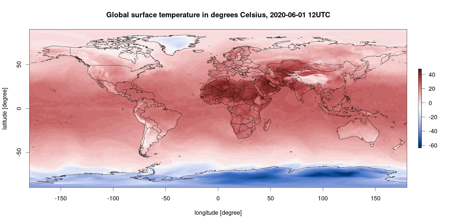
R is also capable of plotting geo-referenced data sets, e.g., spatial data as in this example. This figure shows the surface air temperature in degrees Celsius for March 7, 2018 at 12 UTC (which is 1 pm local time in Central Europe) based on the ECMWF ERA5 reanalysis data set using Copernicus Climate Change Service information.
R packages used: ecmwfr, ncdf4, raster, maps, colorspace.
Some more (mostly) nice spatial R examples can be found on Spatial.ly.
Geographical data
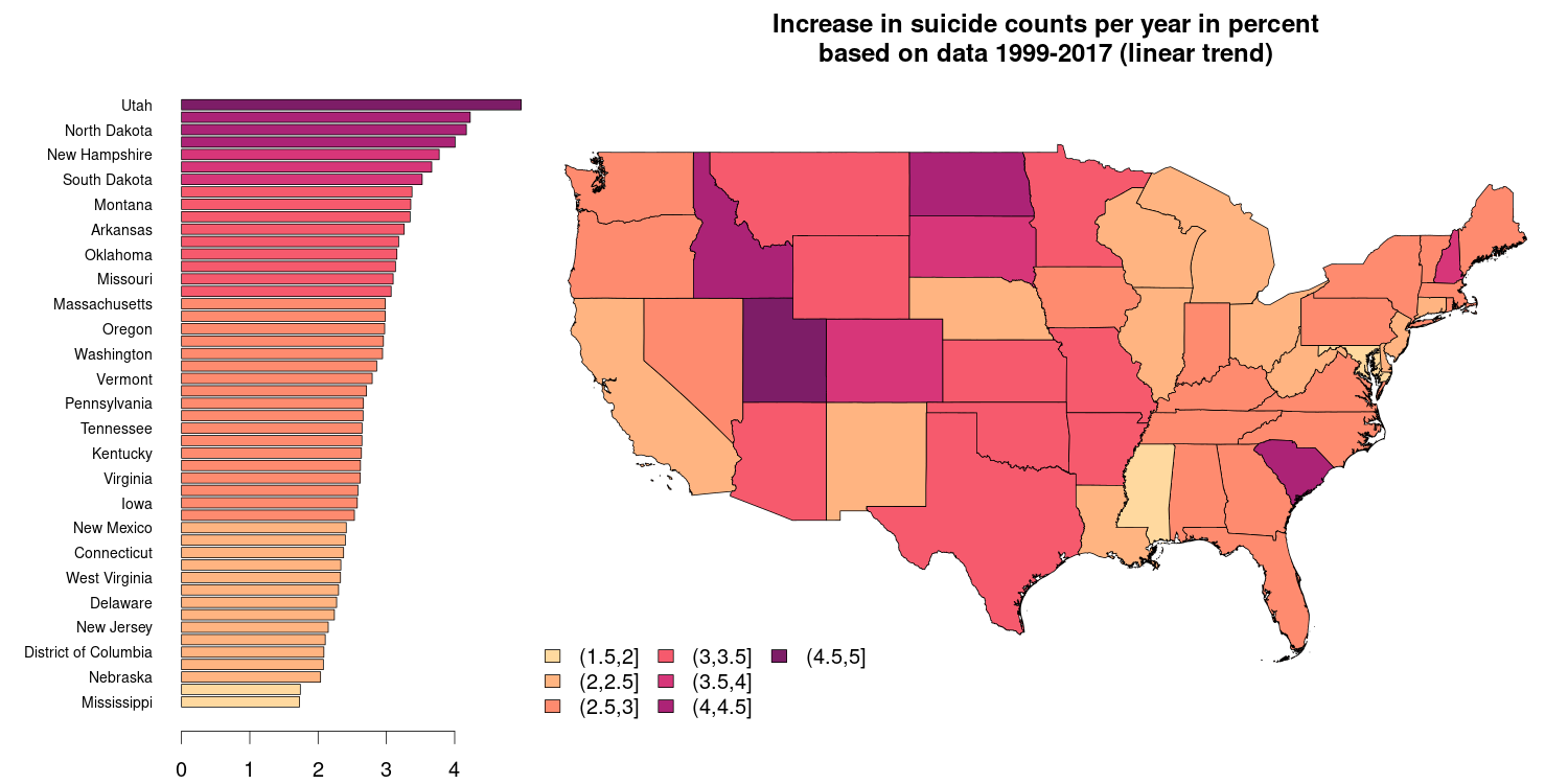
Another common type of visualizations are geo-referenced data on an e.g., national or international level. The figure below is based on a public data set by the National Center for Health Statistics (id bi63-dtpu, csv format) and shows the mean increase in the number of suicides on a state level (excluding Alaska and Hawaii) over the years 1999-2016 in percent. The barplot on the right hand side shows the very same information as the spatial plot on the right hand side.
State boundaries downloaded from the GADM website which provides national/political boundaries in an R format (rds) for different levels of detail (national and sub-national).
R packages used: sp, zoo, colorspace.
For a list of contributed R packages dealing with spatial and spatio-temporal data visit the Spatial and SpatioTemporal CRAN task views. Some more (mostly) nice spatial R examples can be found on Spatial.ly.
Text mining
Beside spatial or geographical data sets R is also often used for text mining applications (automatically classifying texts, find similarities between different texts, study the evolution of language, …).
The example below shows so called word clouds based on the latest 500 tweets (from twitter) from two American politicians, spring 2019. The tweets are downloaded and cleaned (common words as “the” or “A” are removed, URL’s and some special characters or quotes are removed) before counting the frequency of each word. Words which are used more frequent are shown with a larger font size and darker color. Guess who is who?
R packages used: rtweet, tm, wordcloud, colorspace.
The CRAN task view Natural Language Processing (NLP) shows an overview/list of contributed R packages for processing language/words. For some more inspiration of graphical representations of R based text mining applications visit bnosac.be.
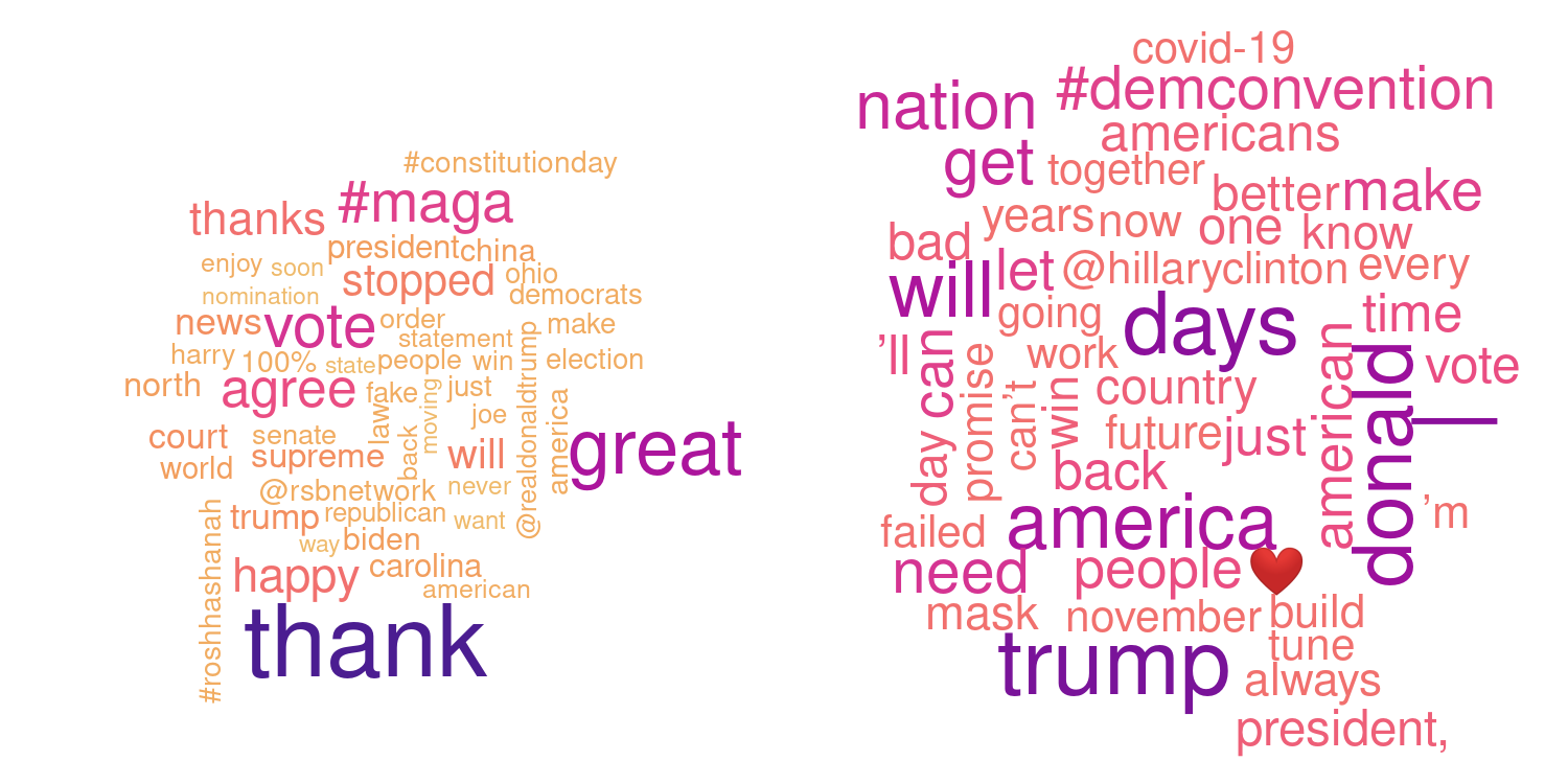
Answer: Donald Trump (left) and Joe Biden (right) based on the latest 550-600 tweets before September 18, 2020.
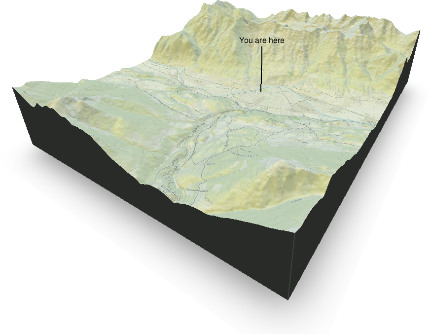
Three-dimensional plots
Three dimensional plots are always a bit more difficult to produce and they often do not make sense (at least not plotting 3D barplots). However, in some cases three dimensional perspective plots can make sense as in this case. The image below shows the area around Innsbruck, a combination of a digital elevation model (ASTER data) and an OpenStreetMap overlay. Takes quite a while to get this result, but looks cool :).
R packages used: OpenStreetMap, rayshader, raster, sp, colorspace.
More details available on the rayshader website.