Chapter 12 Reading & Writing
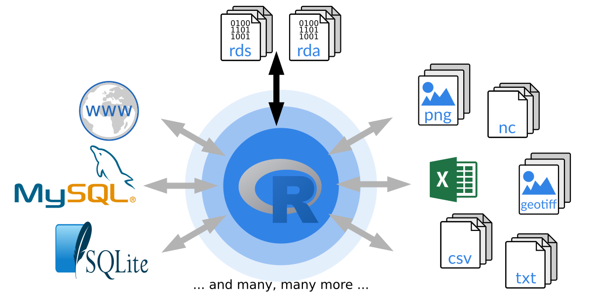
A very important feature of all programming languages is the ability to communicate with the outside world – to import and export data from various sources and formats.
This includes reading and writing simple text files from your local hard disk, download and reading data from the web (e.g., JSON, XML, HTML, …), read and write more complex files like NetCDF or GeoTIFF, spreadsheet files like Excel, select and insert data into data bases, and much more.
In this course we will focus on three topics:
- Introduction to R’s own binary file formats: RDS and RDA and how to store and load objects in these two formats.
- Reading and writing text files with tabular data: CSV-like files.
- A quick introduction on how to read/write XLS/XLSX files.
12.1 Binary vs. text files
In general, we can differ between two main types of data/files. Information is either binary encoded (basically just 0’s and 1’s) or stored in a human readable format as plain text files, sometimes called ASCII files. ASCII stands for ‘American Standard Code for Information Interchange’ and is a standard which dates back to 1963 – today most systems allow for more than the original standard (e.g., different character sets like German Sonderzeichen or Chinese letters) wherefore ‘text files’ is a bit more generic.
Binary files
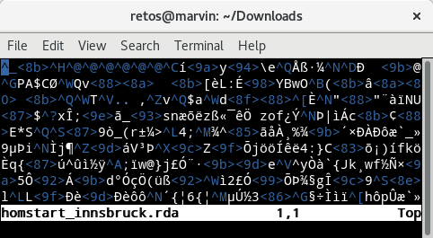
Figure 12.1: Example of a binary file opened in a standard text editor.
The screenshot above shows the content of a binary file opened in a text editor. It shows how my text editor interprets the content of the binary file. For us it is impossible to see what’s in the file.
Binary file properties
- Consist of a series of bytes (i.e., 0/1 bits like
00101011011011). - Not human readable, we ‘need’ a machine to decode the content.
- Lots of standards for different types of data.
- The advantage of binary files: they allow for a much higher compression than text files (less space on hard disk; less bandwidth when browsing/downloading from the internet).
- Often contain some kind of meta-information in the header (to get a clue what is in these files).
- Reading and writing requires specific knowledge of the file format (or existing libraries to encode/decode the data).
Examples for commonly used binary files are e.g., images (PNG, JPG, GIF), archives (ZIP, tar, Gzip), or language-specific file formats (rda/rds in R, pickle (and others) in Python, or mat files in Matlab).
Text files
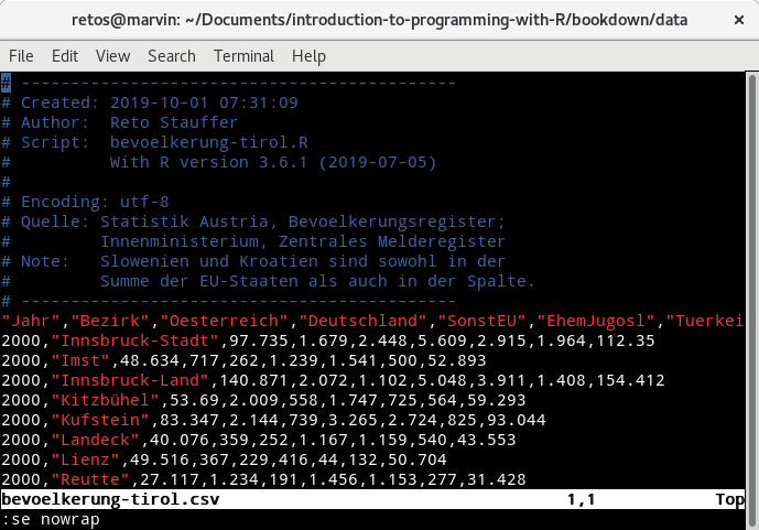
Figure 12.2: Screenshot of a tabular text file opened in a standard text editor.
This is the content of a CSV file represented by a sequence of human readable
characters (or “text”). You can see that the content of the file consists of a
series of comments (blue) followed by a set of values separated by commas (,)
with a column description in the first row after the comment section (a header)
followed by a set of rows containing the actual data.
The first column is called "Jahr" and contains an integer value, the second
one "Bezirk" with the name of a district in Tyrol, and so on (feel free to
download the csv file or the R script
to download and generate the csv file.
Text file properties
- Still stored binary (
00100101), but the bytes correspond do characters. - Standard text-editors convert the binary data into human readable text.
- Basic reading/writing is directly supported by most programming languages.
- Specific formats have conventions for formatting (like CSV discussed later).
- As stored as ‘text’, the file size is much larger compared to the same information stored in a binary file format.
- Some more details for those interested:
- The encoding (mapping) of bytes to characters may matter. E.g., if your Japanese colleague sends you a text file containing Japanese letters, your computer (German/English) may show strange symbols (wrong encoding).
- The first 128 characters are standardized (for all encodings); beyond that all encodings contain different characters (e.g., German Sonderzeichen, Chinese letters, …).
- Common issues: Single-byte (e.g. Latin1) versus multi-byte (e.g., UTF-8) encoding.
- This stuff is getting important quickly, especially when working with NLP (natural
language processing; even
"äöü"can cause problems).
Examples for other text files you may use on a daily basis are e.g., HTML (“websites”), XML, or JSON.
File formats and R
Which file formats can be read by R? Well, technically - all. However, to be able to read binary files R needs to know what to expect. Base R comes with “basic” functionality to handle some common file types, for more advanced or specialized file formats additional packages need to be installed.
R base (including the recommended packages which are installed automatically) comes with:
- R’s own file formats: RDA and RDS.
- The foreign package offers support for data from other statistical systems such as SAS, SPSS, or STATA.
Additional packages (see The R ecosystem) allow to read a wide variety of data formats. The following list is far away from being complete, but might be of interest to you at some point:
- sf, sp: Reading/writing and handling of spatial data (polygons, points, lines).
- raster, stars (early release): Handling of gridded spatial data.
- rjson to read/parse JSON data,
- xml2 to read, parse, manipulate, create, and save xml files,
- png and jpeg: Reading and writing raster images.
- ncdf4: Read and write NetCDF files.
- RSQLite, RMySQL, influxdbr, RPostgres: Reading and writing different data bases.
- haven: Additional support for data from other statistical systems (SAS, SPSS, Stata, …).
For your future:
These packages are often interfaces to system libraries. Thus, these system libraries are required to be able to install the package. Windows/OS X: packages from CRAN are typically pre-compiled, the required libraries come with the package (Windows binaries/OS X binaries). If not, or if you use Linux, these additional libraries have to be installed in advance.
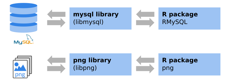
An example: if you visit the
png package website on
CRAN you will see that there is a system requirement,
in this case the libpng library. The package website also shows that, for
Windows and OS X, binaries are available. To be able to install the package on
Linux, libpng and libpng-dev have to be installed. The latter one provide
the header files for compilation.
12.2 RDA and RDS
As most other programming languages, R comes with its own binary format. There are two different types of binary R files for multiple objects (RDA) and for single objects (RDS). Before looking at the functions to read/write, let us first compare the two formats.
For multiple objects: RDA (R data) files.
- File extension (typically):
.rda,.Rda, orRData. - RDA files can take up one or multiple different R objects.
- Preserves the name(s) of the object(s) stored.
load(): Read/load existing files.save(): Write/save data.
For single objects: RDS (serialized R data) files.
- File extension (typically)
.rds, or.Rds. - Can only take up one single object.
- Does not preserve the name of the object saved.
readRDS(): Read/load existing files.saveRDS(): Write/save data.
Note that the file extension is not a hard requirement but highly suggested as
you can easily identify the files as R binary files by name.
In this book we stick to .rda and .rds for files using these two formats.
RDA files
Allows us to easily save and load one or multiple objects at a time. This is very handy if we have to store e.g., several data frames, a data frame and some meta information, a set of functions, or whatever you need to.
Loading RDA files
Usage:
Arguments:
file: Name of the file to load (or a readable binary connection).evnir: Environment where data should be loaded.verbose: Should item names be printed during loading?
Examples
The file argument can be a relative ("data/my_dataset.rda") or an absolute
path (e.g., "C:/Users/Martina/UNI/programming/data/my_dataset.rda").
Note: Try to avoid the use of absolute paths as they will most likely work on
your computer and only as long as you do not re-organize your directories.
If you write a script with absolute paths and send it to a friend, he/she will most likely not be able to run it without adjusting all paths. When using relative paths the code can be written in a way that it works basically everywhere.
Typical problem: If you run into an error "probable reason 'No such file or directory'"
when calling load() check the spelling of the file argument, check if the file
really exists on your computer, and that your working directory is
set correctly. In case you forgot how this worked, check out the
Working directory section in one of the first chapters.
Practical example
As a practical example we will use a file called
demo_file.rda which you can
download (click on file name) and try it at home.
We will first clean up our workspace (remove all existing elements) such that
we can easily see what has been loaded when calling load().
My data set "demo_file.rda" is located inside a directory called "data" inside
my current working directory. Thus, I need to specify the file argument as
"data/demo_file.rda" (might be different on your side).
Nothing is shown/printed when we call the command above. No error (which is
good), but also no output which tells us what the file contained and has been
loaded. One way to see what we got is to call objects() again.
## [1] "info" "persons"As we cleaned the workspace before calling load() these two objects must have
been created by load(). An alternative which I recommend is to set the second
argument verbose = TRUE to get some information about what has been loaded.
## Loading objects:
##   persons
##   info
The two objects persons and info have been crated in our workspace and we
can now start working with them.
##      name height   age gender
## 1  Renate    155 33.07      1
## 2    Kurt    175 22.36      0
## 3 Hermann 171 18.68 0## List of 3
## $ creator: chr "Reto"
## $ date : chr "2020"
## $ note : chr "Demo RDA data set."A last alternative to get the names of the loaded objects is to store the
invisible return of the load() function. load() returns a character string
with the names of the objects loaded. This can become handy when automatically
processing loaded objects at some point.
## chr [1:2] "persons" "info"Summary
- The names are preserved:
load()creates objects with specific names, the names of the objects originally stored in the RDA file. - RDA files can contain multiple R objects.
Writing RDA files
Instead of loading existing RDA files we can save any R object into
an RDA file such as results of an analysis, prepared data sets, estimated
statistical models, or even functions (any object).
This is done using the save() function.
Usage
save(..., list = character(),
     file = stop("'file' must be specified"),
     ascii = FALSE, version = NULL, envir = parent.frame(),
     compress = isTRUE(!ascii), compression_level,
     eval.promises = TRUE, precheck = TRUE)
Important arguments
...: Names of objects (symbols or strings, separated by commas).list: Character vector of object names to be saved (alternative to...).file: File name (or writable binary connection) where data will be saved.version: see notes on the Format version.
Examples
# Save object 'persons' and 'info' into 'persons.rda'
save(persons, info, file = "persons.rda")
# Alternatively via list (character vector!)
save(list = c("persons", "info"), file = "persons.rda")
Practical example
Create yourself two new objects with an integer sequence and a numeric
sequence. Once created, save these two objects into an RDA file and clean your
workspace (rm(list = objects())) to remove all objects. Load the RDA file
again – both objects should be loaded from the data set and re-created in your
workspace.
# Create the two objects
x       <- -10:10
num_seq <- seq(0, 5, 0.1)

# Save the two objects
save(x, num_seq, file = "_testfile.rda")
rm(list = objects())        # Clean workspace
objects()                   # Should return an empty character vector
## character(0)## [1] "num_seq" "x"Note: Alternatively we could also only delete the two objects x and num_seq
instead of clearing the entire workspace by calling rm(x, num_seq) to specifically
delete these two.
## [1] "num_seq" "x"## character(0)RDS files
The handling of RDS files works similar to RDA files with one small but crucial difference: only one single object can be stored, and the name of the object is not preserved. This may sound as a disadvantage at the first sight (we lose the original object name), but is actually extremely convenient.
Reading RDS files
Instead of using load() as for RDA files, we will now use readRDS().
Usage
Important arguments
file: File name or connection where the R object is read from.
Example
Note that there is one important difference to load(). When calling readRDS()
the object loaded from the RDS file is returned after reading the binary file.
Thus, we need to assign (<-) the return to an object. If not, the object
will be printed but not stored, wherefore you can’t use it afterwards.
As mentioned, this can be very handy as we do not have to remember the name of the object we stored as we will assign it to a new custom object with a new (known) name. When working with RDA files you need to remember how the objects were called, or develop code that auto-detects what the original name was.
Practical exercise
You can download the demo_file.rds
to try it out on your own. Again, take care about the position of the file on your
system such that R can find and read the file when calling readRDS().
My file is, again, located in a directory "data" inside my current working
directory, wherefore the file name is "data/demo_file.rds" in my case.
If we don’t assign the return of readRDS() to a new object, the data set
will automatically be printed. Thus, we assign the return to a new object
which I call data.
##      name height   age gender
## 1  Renate    155 33.07      1
## 2    Kurt    175 22.36      0
## 3 Hermann    171 18.68      0
## 4    Anja    152 18.96      1
## 5  Andrea    165 45.52      1
## 6  Bertha    155 24.40      1
The object loaded is the same as we had in the RDA file and was originally
called persons.
However, when working with RDS the object names are not
preserved and we do not have to know what the original name was. We simply
assign the return to a new object (here data) and are then able to proceed
with this object. Job done.
# Reading multiple times
x1 <- readRDS("data/demo_file.rds")
x2 <- readRDS("data/demo_file.rds")
identical(x1, x2)
## [1] TRUEIf loaded multiple times and stored on different objects
(x1, x2) both objects are, of course, identical.
Writing RDS files
This is very straight forward as well. Instead of using save() as for RDA
files we call the saveRDS() function.
Usage
Important arguments
object: your R object to serialize (only one).file: name of the file (or a writable binary connection) where to store the object.version: see notes on the Format version.
Examples
Note that something as follows is not possible!
Practical exercise
Very simple example where we create a simple integer sequence x which we then
store into an RDS file and load it again.
x <- -4:4
saveRDS(x, "_integer_sequence_demo.rds")
# Load and store on y
y <- readRDS("_integer_sequence_demo.rds")
# Are 'x' and 'y' identical?
identical(x, y)
## [1] TRUEAdvanced use of RDS files
To show that RDS files can be very handy, let us do another example. Imagine you do a survey. You ask different people a series of questions and would like to store the results (answers) in separate RDS files.
For this purpose three simple data frames will be created and written into three separate RDS files in the next code chunk.
# Data of person/subject A
personA <- data.frame(name = "Jessica", department = "Botany",
                      semester = 4, age = 22, distance_to_university = 10.3)
# Data of person/subject B
personB <- data.frame(name = "Frank", department = "Organic Chemistry",
                      semester = 7, age = 24, distance_to_university = 1.0)
# Data of person/subject C
personC <- data.frame(name = "Mario", department = "Geology",
                      semester = 6, age = 28, distance_to_university = 3.2)

# Save data
saveRDS(personA, "_survey_results_A.rds")
saveRDS(personB, "_survey_results_B.rds")
saveRDS(personC, "_survey_results_C.rds")
Once stored we can now load the objects again – one by one – if needed.
##      name department semester age distance_to_university
## 1 Jessica     Botany        4  22                   10.3
What if we would like the content of multiple files at once? Remember the
*apply() functions from one of the previous chapters
(see Apply functions)?
*apply() also work on character vectors.
We create a character vector files with the names of the three
files we want to load and use lapply() to read all three files.
## [1] "_survey_results_A.rds" "_survey_results_B.rds" "_survey_results_C.rds"## [[1]]
## name department semester age distance_to_university
## 1 Jessica Botany 4 22 10.3
##
## [[2]]
## name department semester age distance_to_university
## 1 Frank Organic Chemistry 7 24 1
##
## [[3]]
## name department semester age distance_to_university
## 1 Mario Geology 6 28 3.2## name department semester age distance_to_university
## 1 Jessica Botany 4 22 10.3
## 2 Frank Organic Chemistry 7 24 1.0
## 3 Mario Geology 6 28 3.2Don’t worry: We never heard about do.call() and you don’t need
to know it, but it can be used to apply a function (here rbind)
on a series of elements of a list (data). In this case we use
row-bind the three data frames from the three files.
Format version
A side-note which may not be crucial for you during this course, but something you should keep in mind, especially when collaborating with colleagues and/or if you run scripts on multiple computers/servers where the R may have been updated to a newer version.
Between R version \(3.5\) and \(3.6\) the default binary file format of rds/rda files has changed. In the “old” days R was using format version \(2\), now (since R \(3.6\)) the default is format version \(3\).
- R \(< 3.5\) uses
version = 2by default, can not readversion = 3 - R \(\equiv 3.5\) uses
version = 2by default, can readversion = 3 - R \(> 3.6\) uses
version = 3by default, can read/writeversion = 2(backwards compatibility)
Thus, if you store an rda/rds file from R \(\ge 3.6\) it will, by default, be stored in format version \(3\). These files cannot be read by old R installations (R version \(< 3.5\)).
It his highly recommended to update the R version as \(3.4\) is already pretty old. However, if not possible, we can also always store rda/rds files in the older format version \(2\) as follows:
# Create test matrix
mymat <- matrix(1:9, nrow = 3)
# Testing version2/3
save(mymat, file = "testfile_v2.rda", version = 2)
load("testfile_v2.rda", verbose = TRUE)
## Loading objects:
## mymatNote: when loading (load(), readRDS()) we do not have to specify the
format version. R will automatically detect the version.
To check your current R version, call R.version.
12.3 Reading CSV
Let us move from binary files to text files. This section will cover one specific type of text files containing tabular data. We have already seen a screenshot of how such a file can look like in a text editor:
You can think of it as a “data frame” or “matrix” stored in a plain text file, where each row contains an observation, the different values are separated by a separator (above by commas). This is a common way to store and exchange data sets as they are easy to read (human readable) and relatively easy to load and save.
Disadvantages: The devil is in the detail.
- Different files have different column separators: Commas, semicolon, tab, space, …
- Different decimal separators depending on language:
.vs.,(1.5vs.1,5). - Can contain variable names in the first row (header;header; optional).
- Coding of missing values might differ:
NA,NaN,-999,missing, … - Some frequently used relatively well-defined formats exist, however, there is no real standard.
- Character encoding of the files may differ: ASCII, Latin1, UTF-8, …
Speaking of weak standards: Such files will often be called
CSV
files where CSV stands for “Comma Separated Values”. While there is some kind
of standard for CSV files, these standards are not very strict. While English
speaking countries really use commas to separate values (thus CSV) this is a
problem for most European locales (languages) as they use the , for the
decimal separator of numeric values (e.g., 20,43; decimal comma). Thus,
instead of a comma to separate the values, a semicolon (;) is used. However,
files with this format are still considered as ‘CSV’.
Reading functions
The workhorse in R to read such tabular data from text files is the function
read.table() (details later) alongside with a series of convenience interfaces.
Defaults
| Function | Separator | Decimals | Header |
|---|---|---|---|
read.table() |
“White space” (space or tab) | point | no |
read.csv() |
Comma-separated | point | yes |
read.csv2() |
Semicolon-separated | comma | yes |
read.delim() |
Tab-separated | point | yes |
read.delim2() |
Tab-separated | comma | yes |
All functions are based on read.table() but have somewhat different defaults
for common tabular data files. These defaults can, of course, be changed if needed.
“Standard” CSV file
The output below shows the first few lines of the file homstart-innsbruck.csv (click for download) and contains monthly average temperatures and monthly precipitation sums for innsbruck since the year 1952.
This CSV file is closest to the originally proposed standard using a comma as value separator and a decimal point for floating point numbers.
"year","month","temperature","precipitation"
1952,"Jan",-6,54.3
1952,"Feb",-2.8,67.6
1952,"Mar",3.7,55.5
1952,"Apr",11.1,37.1
The first line contains the header (names of variables in the columns), in this
case year, month, temperature (\(^\circ C\)) and precipitation (liter per \(m^{2}\)).
All following lines contain one observation per line, all values separated by a
comma. Character strings (header, month names) are quoted ("...").
Remark: The content below shows the first lines of the file homstart-innsbruck.dat which is also considered as a valid CSV file. However, it is a bit further away from the original CSV ‘standard’.
- Contains additional comments (meta-information).
- Uses a different file extension (
.dat). - The value separator is a semicolon (
;). - Uses decimal comma.
- Strings are not quoted (not
"...").
# Meta information: Weather data, Innsbruck
# year:   year of observation
# month:  month of observation
# temp:   monthly mean temperature
# precip: monthly accumulated precipitation sum
year;month;temperature;precipitation
1952;Jan;-6;54,3
1952;Feb;-2,8;67,6
1952;Mar;3,7;55,5
1952;Apr;11,1;37,1
Reading CSV
Usage
read.csv(file, header = TRUE, sep = ",", quote = "\"",
         dec = ".", fill = TRUE, comment.char = "", ...)
read.csv2(file, header = TRUE, sep = ";", quote = "\"",
          dec = ",", fill = TRUE, comment.char = "", ...)
Arguments
- Note: Main difference between the two functions are somewhat different default arguments.
file: File name or connection or URL with data to be read.header: Is there a header line with the variable/column names?sep: Column separator.quote: Quoting characters.dec: Decimal separator.fill: Should incomplete lines be filled with blanks?comment.char: Character indicating rows with comments....: Further arguments passed toread.table().
Example: We will read the two files
homstart-innsbruck.csv
(“standard” CSV) and
homstart-innsbruck.dat
(nonstandard CSV) using the two functions read.csv() and read.csv2().
As the first file is in the ‘standard format’ as expected by read.csv() all
we have to do is to call:
##   year month temperature precipitation
## 1 1952   Jan        -6.0          54.3
## 2 1952   Feb        -2.8          67.6
## 3 1952 Mar 3.7 55.5## 'data.frame': 672 obs. of 4 variables:
## $ year : int 1952 1952 1952 1952 1952 1952 1952 1952 1952 1952 ...
## $ month : chr "Jan" "Feb" "Mar" "Apr" ...
## $ temperature : num -6 -2.8 3.7 11.1 12.8 16.7 19.3 18.1 11.4 7.3 ...
## $ precipitation: num 54.3 67.6 55.5 37.1 75.6 ...The return is a named data frame using the first line of the file as
variable/column names (header = TRUE). How can we read the second
file (.dat)? As shown above, this file has additional comments,
uses semicolons as separator, and a decimal comma. When checking
the defaults of read.csv2() we can see that that’s mostly the
defaults of the function (sep = ";", dec = "."). What’s missing
is a character which defines lines with comments which we have
to specify in addition.
## year month temperature precipitation
## 1 1952 Jan -6 54.3We could, of course, also use read.csv() and specify all arguments
in the way needed to read this second file:
data <- read.csv("data/homstart-innsbruck.dat",
sep = ";", dec = ",", comment.char = "#")
head(data, n = 2)## year month temperature precipitation
## 1 1952 Jan -6.0 54.3
## 2 1952 Feb -2.8 67.6Missing values
What about missing values? The default is na.strings = "NA".
Whenever the text file contains the letters NA or "NA" they
will be automatically replaced by a missing value (NA in R).
If our text file contains a different string for missing values,
we can specify them using the na.strings argument. na.strings
takes up a character vector with all elements which should be
replaced by NA. Let us have a look at the following file
called homstart-missing.csv
(click to download):
"year","month","temp","precip"
1952,"Jan",-6,NA
1952,"Feb",-999,10.5
1952,"Mar",55,
1952,"Apr",,35.2The file contains several different missing-value strings, namely
.NA, "" (empty strings), and -999 (value indicating a missing observation).
We can replace all these values while reading by calling:
## year month temp precip
## 1 1952 Jan -6 NA
## 2 1952 Feb NA 10.5
## 3 1952 Mar 55 NA
## 4 1952 Apr NA 35.2An important detail: R versions previous to 4.0 used different defaults.
There is an argument stringsAsFactors (handled by read.table()) which
controls if columns containing characters should automatically be converted
to factor columns when reading the file. Before 4.0 the default was stringsAsFactors = TRUE,
with \(\ge\) 4.0 the default became FALSE. This might be something you
have to consider if you use existing R scripts/code or a computer with
an old R installation. See the difference:
## 'data.frame':    672 obs. of  4 variables:
##  $ year         : int  1952 1952 1952 1952 1952 1952 1952 1952 1952 1952 ...
##  $ month        : chr  "Jan" "Feb" "Mar" "Apr" ...
##  $ temperature  : num  -6 -2.8 3.7 11.1 12.8 16.7 19.3 18.1 11.4 7.3 ...
## $ precipitation: num 54.3 67.6 55.5 37.1 75.6 ...## 'data.frame': 672 obs. of 4 variables:
## $ year : int 1952 1952 1952 1952 1952 1952 1952 1952 1952 1952 ...
## $ month : Factor w/ 12 levels "Apr","Aug","Dec",..: 5 4 8 1 9 7 6 2 12 11 ...
## $ temperature : num -6 -2.8 3.7 11.1 12.8 16.7 19.3 18.1 11.4 7.3 ...
## $ precipitation: num 54.3 67.6 55.5 37.1 75.6 ...Using read.table()
As mentioned in the beginning, read.csv() and read.csv2() are
convenience functions, the actual work of reading the text files
is always done by the function read.table(). When looking at the
usage of this function we can see that read.table() allows for
a much higher level of customization (most arguments can also
be passed to read.csv() and read.csv2() if needed).
Usage
read.table(file, header = FALSE, sep = "", quote = "\"'",
           dec = ".", numerals = c("allow.loss", "warn.loss", "no.loss"),
           row.names, col.names, as.is = !stringsAsFactors,
           na.strings = "NA", colClasses = NA, nrows = -1,
           skip = 0, check.names = TRUE, fill = !blank.lines.skip,
           strip.white = FALSE, blank.lines.skip = TRUE,
           comment.char = "#",
           allowEscapes = FALSE, flush = FALSE,
           stringsAsFactors = default.stringsAsFactors(),
           fileEncoding = "", encoding = "unknown", text, skipNul = FALSE)
Some important arguments
nrows: Read onlyNlines (default-1; all).skip: Skip the firstNlines (default0).strip.white: Remove leading/trailing white spaces from characters.blank.lines.skip: Ignore blank lines.fileEncoding: Character set used for encoding (e.g.,"UTF-8","latin1", …).text: Read from a character string rather than a file.
Example: This allows us to read even more custom files. The file names.csv contains the following:
------
name: names.csv
author: reto
-----


name, age, location
Paul

Peter, 35, Vienna
Verena, 23,
Klaus,, Paris
A pretty ugly file, however, we can still read it using the correct arguments. What do we have to consider?
- Ignore the first 4 lines (
skip = 4) as they are not part of the data. - Skip empty lines (
blank.lines.skip = TRUE; default). - We do have a header with column names (
header = TRUE). - The separator is a comma (
sep = ","). - fill in missing elements (
fill = TRUE; e.g., in the line forPaul).
read.table("data/names.csv",
           skip = 4,
           blank.lines.skip = TRUE,
           header = TRUE,
           sep = ",",
           fill = TRUE)
## name age location
## 1 Paul NA
## 2 Peter 35 Vienna
## 3 Verena 23
## 4 Klaus NA ParisTechnically also possible via the read.csv() function, try to replace
read.table() with read.csv(): do you get the same?
Exercise 12.1 Let us try to do something cool with the data set.
Download the data
set and read it using read.csv()
Store the return on an object clim as above.
- What is the average (mean) January temperature in Innsbruck?
- What is the average (mean) temperature in July?
- Could we do (1) and (2) dynamically? Try to calculate the monthly average temperature for each month using a for loop.
- Try to create a boxplot which shows the climatology, namely plotting “temperature” (y axis) against the name of the month (x axis).
Solution. Import/read data set
# Read file (your path/file name may differ, of course)
clim <- read.csv("data/homstart-innsbruck.csv")
(1) Average January temperature
One way to solve this is to subset the data.frame such that it only
contains data for January. I’ll store this subset on a new object called
clim_jan:
## [1] 56 4Once we have the subset, we can simply calculate the average temperature
using mean() on the variable temperature as follows:
## [1] -1.992857(2) Average temperature in July
Just the very same:
## [1] 18.4625(3) Calculate mean temperature for all months
Instead of manually calculating the average temperature we could also
try to solve this dynamically. E.g., using a loop over all the
months in the data set:
# Looping over all unique values in clim$month (each month)
months <- unique(clim$month)
for (m in months) {
    # Calculate average temperature
    avg <- mean(subset(clim, month == m)$temperature)
    # Round the average temperature, 1/10th of degrees
    avg <- round(avg, 1)
    cat("Average monthly mean temperature for", m, "is", avg, "\n")
}
## Average monthly mean temperature for Jan is -2
## Average monthly mean temperature for Feb is 0.4
## Average monthly mean temperature for Mar is 5.2
## Average monthly mean temperature for Apr is 9.1
## Average monthly mean temperature for May is 13.7
## Average monthly mean temperature for Jun is 16.8
## Average monthly mean temperature for Jul is 18.5
## Average monthly mean temperature for Aug is 17.9
## Average monthly mean temperature for Sep is 14.7
## Average monthly mean temperature for Oct is 9.9
## Average monthly mean temperature for Nov is 3.6
## Average monthly mean temperature for Dec is -1.1Let’s try to do the same using the loop replacement function sapply():
# Custom function to calculate average temperature
# First input will be the 'level' (month name; x)
# We also provide a 'data' argument with our object 'clim'
calc_avg_temp <- function(x, data) {
    # Take the subset first
    data <- subset(data, month == x)
    # Calculate and return the average temperature
    return(round(mean(data$temperature), 1))
}

# Call the function using sapply()
sapply(unique(clim$month), FUN = calc_avg_temp, data = clim)
## Jan Feb Mar Apr May Jun Jul Aug Sep Oct Nov Dec
## -2.0 0.4 5.2 9.1 13.7 16.8 18.5 17.9 14.7 9.9 3.6 -1.1(4) Create climatology boxplot
All we have to do is to tell R to create a boxplot(). We can
use the “formula interface” and just specify that we would like to
have temperature ~ month (temperature explained by month):
boxplot(temperature ~ month, data = clim,
        main = "Temperature Climatology Innsbruck",
        ylab = "mean monthly temperature [C]")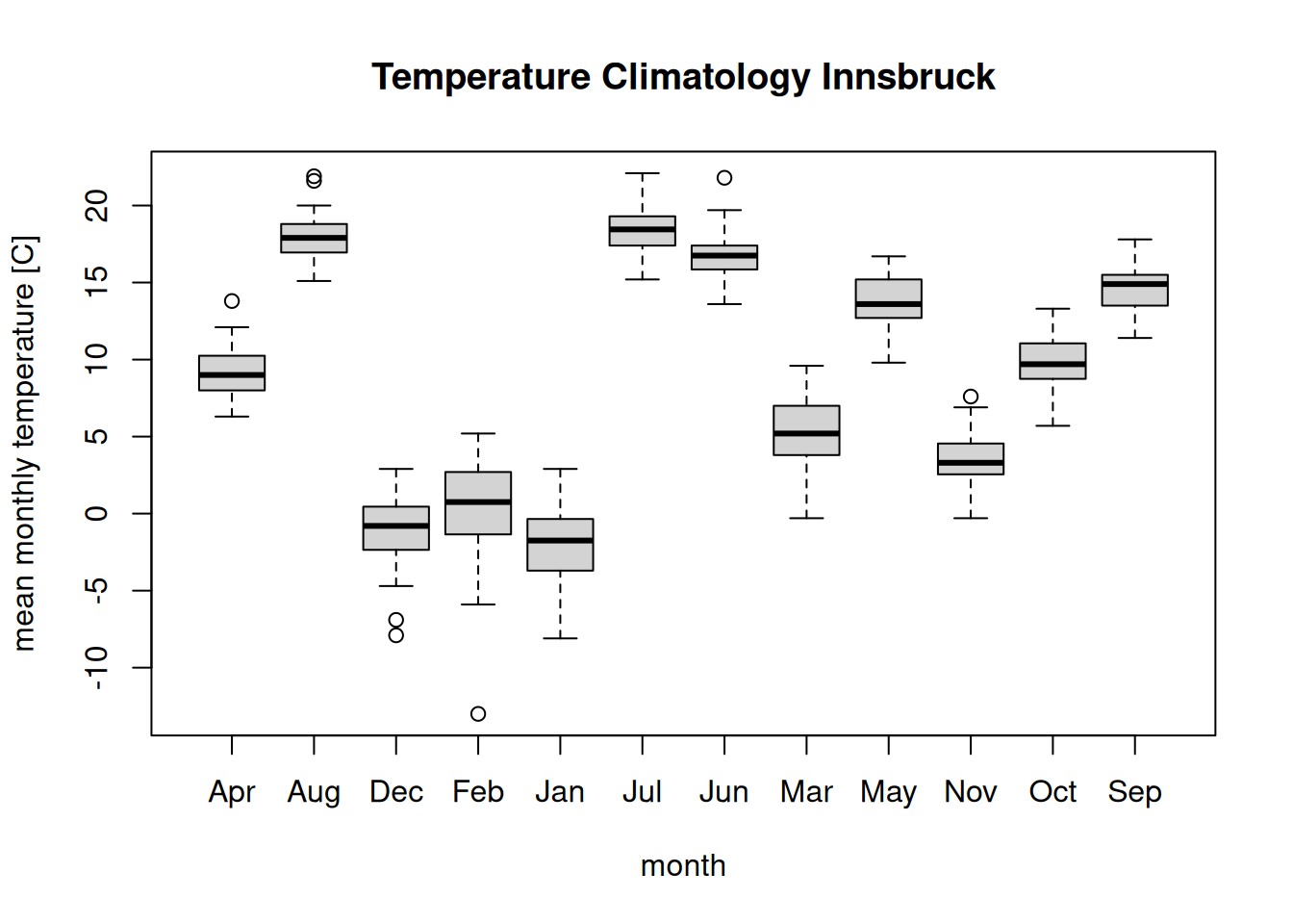
The problem: The order of the months is completely off. The reason is
that temperature ~ month internally converts month into a factor
variable to be able to create the plot. As we know, as.factor(...)
orders the levels lexicographically (Apr, Aug, …, Sep). To get
the correct we could create a proper factor ourself before doing the plot …
clim$month <- factor(clim$month, month.abb)
levels(clim$month) # Correct order as defined by month.abb
## [1] "Jan" "Feb" "Mar" "Apr" "May" "Jun" "Jul" "Aug" "Sep" "Oct" "Nov" "Dec"… and call the boxplot() function once again.
boxplot(temperature ~ month, data = clim,
        main = "Temperature Climatology Innsbruck",
        ylab = "mean monthly temperature [C]")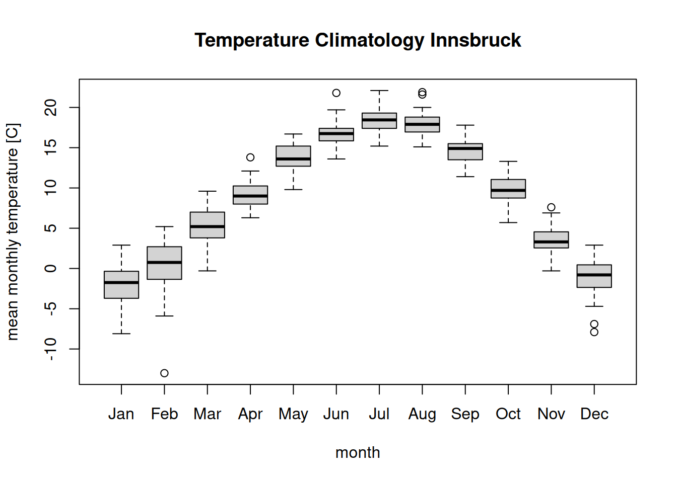
12.4 Writing CSV
Instead of only reading CSV files we can also write CSV-alike files.
The functions work analogously to the reading functions and come with a
wide range of arguments which can be set, check ?write.table for details.
write.table(): Workhorse function.write.csv(),write.csv2(): Convenience interfaces with adapted defaults.
The first input argument to write.table() and write.csv() is the object
we would like to store, preferably a data frame or matrix.
Examples Let us use the “Innsbruck” data set. We first load the content of the file homstart-innsbruck.csv and write it into a new text file.
The content of the text file then looks as follows.
"","year","month","temperature","precipitation"
"1",1952,"Jan",-6,54.3
"2",1952,"Feb",-2.8,67.6
"3",1952,"Mar",3.7,55.5
"4",1952,"Apr",11.1,37.1
Row names
Noticed the additional first column? Well, by default, the row names
are also written into the output file! That’s nothing else as rownames(data1)
of our original data frame. If we would not read the file again we get the
following object:
##   X year month temperature precipitation
## 1 1 1952   Jan        -6.0          54.3
## 2 2 1952   Feb        -2.8          67.6
## 3 3 1952   Mar         3.7          55.5
## 4 4 1952   Apr        11.1          37.1
The additional column X contains the row names (as separate column).
We can tell write.csv() and write.table() to not write these uninformative
row names into the text file by setting the argument row.names = FALSE.
"year","month","temperature","precipitation"
1952,"Jan",-6,54.3
1952,"Feb",-2.8,67.6
1952,"Mar",3.7,55.5
1952,"Apr",11.1,37.1
An alternative way is to tell R that a specific column in the text file
contains row names. This might be important if you have an object with
informative row names. Let us write our data1 into the file "data1.csv" once
again leaving row.names = TRUE and read the text file twice:
- Once without additional arguments: Gives us the extra
Xcolumn. - Once specifying
row.names = 1: Expects that the first column contains row names.
write.csv(data1, "data1.csv")
d1 <- read.csv("data1.csv")
d2 <- read.csv("data1.csv", row.names = 1)
head(d1, n = 3)
## X year month temperature precipitation
## 1 1 1952 Jan -6.0 54.3
## 2 2 1952 Feb -2.8 67.6
## 3 3 1952 Mar 3.7 55.5## year month temperature precipitation
## 1 1952 Jan -6.0 54.3
## 2 1952 Feb -2.8 67.6
## 3 1952 Mar 3.7 55.5If row.names is an integer, it defines the column containing the row names. If
character, the column with this specific name will be used as rownames on the return
of the function.
Exercise 12.2 A small example to write a matrix and a data frame into a text file (CSV file). First, create the following two objects:
# Create a data.frame (city, population, flag for 'city has a metro')
(my_df <- data.frame(city        = c("Innsbruck", "Moscow", "Dallas"),
                     population  = c(132493, 12506468, 1197816),
                     has_metro   = c(FALSE, TRUE, FALSE)))
## city population has_metro
## 1 Innsbruck 132493 FALSE
## 2 Moscow 12506468 TRUE
## 3 Dallas 1197816 FALSE# Create the matrix
(my_matrix <- matrix(1:9, ncol = 3L,
dimnames = list(LETTERS[1:3], letters[1:3])))## a b c
## A 1 4 7
## B 2 5 8
## C 3 6 9The exercise:
- Write the two objects in two separate CSV files.
- Feel free to use
write.csv(),write.csv2(), orwrite.table(). Or try different versions to see where the differences are. - Data frame:
- Don’t write row names into the CSV file.
- Open the CSV file with a text/code editor and check the content.
- Read the new file and store the return on
my_df2. - Are
my_dfandmy_df2identical?
- Matrix:
- As the row names are informative, write them into the CSV file.
- Open the CSV file with a text/code editor and check the content.
- Read the newly created file, take care of proper row name handling,
and store the return on
my_matrix2. - Is
my_matrix2identical tomy_matrix?
Solution. Step 1: Write the two objects into a CVS file. This solution
uses write.csv(), but it would work the same way with write.table()
and/or different arguments if needed.
# Write to csv
write.csv(my_matrix, file = "my_matrix.csv")
write.csv(my_df, file = "my_df.csv", row.names = FALSE)Content of the files: The two files should look as follows.
"city","population","has_metro"
"Innsbruck",132493,FALSE
"Moscow",12506468,TRUE
"Dallas",1197816,FALSE"","a","b","c"
"A",1,4,7
"B",2,5,8
"C",3,6,9Reading the two files: Using read.csv() as we also used write.csv().
Note that we have not written any row.names in "my_df.cs" and thus don’t
need to take that into account. However, "my_matrix.csv" contains the
original row names and we would like to read them as row names again (directly).
##        city population has_metro
## 1 Innsbruck     132493     FALSE
## 2    Moscow   12506468      TRUE
## 3 Dallas 1197816 FALSE## a b c
## A 1 4 7
## B 2 5 8
## C 3 6 9Identical return: Are the two new objects identical or at least equal to the original ones?
## [1] FALSE## [1] TRUE## 'data.frame': 3 obs. of 3 variables:
## $ city : chr "Innsbruck" "Moscow" "Dallas"
## $ population: num 132493 12506468 1197816
## $ has_metro : logi FALSE TRUE FALSE## 'data.frame': 3 obs. of 3 variables:
## $ city : chr "Innsbruck" "Moscow" "Dallas"
## $ population: int 132493 12506468 1197816
## $ has_metro : logi FALSE TRUE FALSEThe data frames are not identical, but equal. If you check the two objects
you can see that the original my_df contains an integer column, while
my_df2 now contains a numeric variable. Thus, not identical, but same
information (equal).
And in case of the matrix? Well, they can’t be identical as read.csv() always
returns a data frame. identical() is also testing for the class and can therefore
not be TRUE. What if we convert my_matrix2 into a matrix?
##   a b c
## A 1 4 7
## B 2 5 8
## C 3 6 9## [1] TRUE## [1] TRUEEt voila.
Write “custom” CSV
We can also customize the format of CSV files we write to disk (to a certain
extent). For details check the R documentation for ?write.table.
As an illustrative example we use the following data frame.
(data <- data.frame(manufacturer = c("BMW", "Opel", "Nissan", "", "BMW"),
                    model        = c("Isetta", "Manta", "Micra", "baby horse", "M3"),
                    horsepower   = c(9.5, 80, NA, 0.5, 210),
                    weight       = c(500, NA, 630, 73, 1740),
                    color        = c("blue", NA, "red", "black", NA),
                    wheels       = c(4, NA, 4, NA, 4)))
## manufacturer model horsepower weight color wheels
## 1 BMW Isetta 9.5 500 blue 4
## 2 Opel Manta 80.0 NA <NA> NA
## 3 Nissan Micra NA 630 red 4
## 4 baby horse 0.5 73 black NA
## 5 BMW M3 210.0 1740 <NA> 4By specifying a series of custom arguments we can take relatively detailed control on how the output format looks like.
write.table(data, "custom_output_format.dat",
            sep = "|", quote = FALSE, dec = ",",
            row.names = FALSE, na = "MISSING")
manufacturer|model|horsepower|weight|color|wheels
BMW|Isetta|9,5|500|blue|4
Opel|Manta|80|MISSING|MISSING|MISSING
Nissan|Micra|MISSING|630|red|4
|baby horse|0,5|73|black|MISSING
BMW|M3|210|1740|MISSING|4To read it again, we of course need to specify the format appropriately:
read.table("custom_output_format.dat", header = TRUE,
           sep = "|", dec = ",", quote = "", na.strings = "MISSING")
## manufacturer model horsepower weight color wheels
## 1 BMW Isetta 9.5 500 blue 4
## 2 Opel Manta 80.0 NA <NA> NA
## 3 Nissan Micra NA 630 red 4
## 4 baby horse 0.5 73 black NA
## 5 BMW M3 210.0 1740 <NA> 412.5 Excel spreadsheets
Another widely used file format for data exchange are Excel spreadsheet files. We can, of course, also read and write XLS/XLSX files - but not with base R. Additional packages are needed to be able to read and write this format.
Formats
- XLS: Proprietary binary file format (until 2007).
- XLSX: Office Open XML, an open XML-based format. XLSX files are technically ZIP-compressed XML documents (2007+).
Advantages: A widely used format for data tables (“sheets”) along with computations, graphics, etc.
Disadvantages:
- Old XLS format is proprietary and changed across different Excel versions. Thus, not always easy/possible to read.
- Both XLS and XLSX can be hard to read due to heterogeneous content.
- There is no standard open-source implementation, but many tools with different strenghts and weaknesses.
Comparison: XLS/XLSX vs. CSV.
- The flexibility of spreadsheet formats encourage some users to add potentially extraneus content that makes it unnecessarily hard to read (with a programming language).
- CSV files have a much more restricted format and are typically relatively easy to read (with a program).
- Hence, the adoption of CSV-based workflows is recommended if possible/applicable. This is of course not always the case, but if you can avoid spreadsheets try to avoid them, it will make your life much easier!
The screenshot below shows an example of an XLSX file. Sure, this is something made up for this book, but it is less far away from reality as you may think. People do strange things if they can/the software allows them to do so. If someone comes around the corner with such a file and ask something like “Hey, I heared you are good at programming, I have an Excel file with some data. Could you quickly read it …” and the file looks somewhat like the one below – RUN!
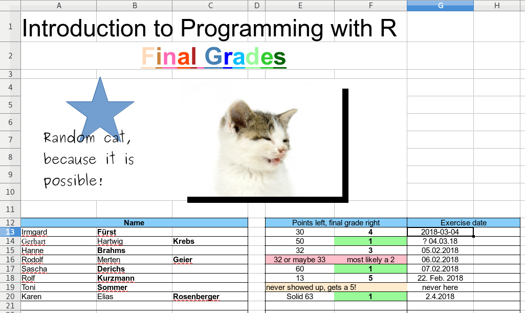
This is a highly complicated format and not easily machine readable. Beside the unnecessary artistic first part the data is also stored in a very complicated way.
- We have two separate tables instead of one.
- The family names are sometimes in column B, sometimes in C.
- Not all columns have a name or label.
- Several cells are merged (combined).
- Columns E/F are mixed numerics and text (natural language is used). Sometimes even merged containing information about points and grade.
- The date comes in at least 4 different formats.
In other words: it is basically impossible to automatically read and process the information in this spreadsheet using custom code. In contrast, the screenshot below shows a well-formatted spreadsheet.
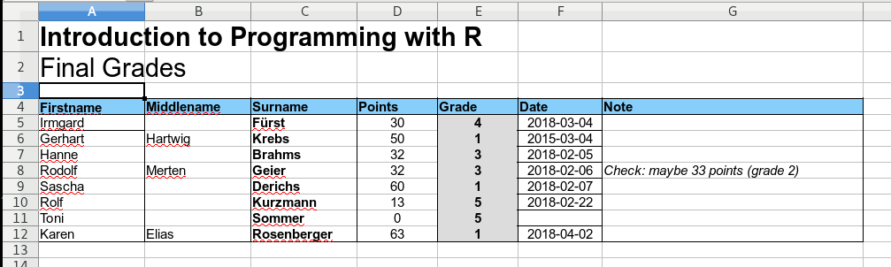
This files comes in a nice machine-readable format.
- One table, all columns are properly named.
- The information is stored in the correct columns.
- Points/grade contain proper numeric values.
- The date format is always the same.
- Additional notes are in an extra column.
When using spreadsheet files and you plan to process the data automatically, try to stick to a simple and very well structured format without a lot of fancy features, else you’ll spend hours to write code to extract the information (or to re-write the entire spreadsheet document) before being able to start processing the data.
Reading spreadsheets
R base has no support for reading this file format. However, a series of additional packages exist on CRAN which allow to read and/or write XLS/XLSX files. However, all these packages come with some strengths and weaknesses.
gdata:read.xls()for reading XLS and (some) XLSX files (cannot write XLS/XLSX).- Arguments as in
read.table(). - Requires Perl at runtime (see perl.org).
openxlsx:read.xlsx()andwrite.xlsx()for reading/writing XLSX.- Some arguments differ from
read.table(). - Employs C++, but binaries are available via CRAN.
readxl:read_excel()for reading both XLS/XLSX (cannot write XLS/XLSX).- Arguments differ from
read.table()but are similar as inreadr(returning tibble data frames). - Employs C++, but binaries are available via CRAN.
xlsx:read_excel()for reading both XLS/XLSX (cannot write XLS/XLSX).- Arguments differ from
read.table()and require sheet index (or name). - Requires Java at runtime.
writexl: Allows to write XLS. Employs C librarylibxlsxwriter, binaries available via CRAN.WriteXLS:WriteXLS()for writing both XLS/XLSX. Requires Perl at runtime.XLConnect: Functionality for querying and manipulating (including reading/writing) spreadsheets. Requires Java at runtime.
Read an XLSX file
The readxl package
is not automatically installed. To be able to use it, we once need to install it by
calling install.packages("readxl") which is downloading the package from
CRAN and installs it into your package library. Once installed
(must be done only once) we can load the library and use its functionality.
Note that the readxl no longer returns data frames when reading XLS/XLSX files,
but a “tibble data frame” (see tibble).
Similar to data frames and can always be coerced to data frames (as.data.frame()) if needed.
The demo file “demofile.xlsx” contains
the cat-example and the well-formatted version also shown above.
We can use the readxl package to read the content of this XLSX file as follows:
# Loading the readxl library
# Required to be able to use the additional functions.
library("readxl")
# Reading the xlsx file
data <- read_xlsx("data/demofile.xlsx",  # name of the file
                  sheet = "good",        # which sheet to read
                  skip = 3)              # skip first 3 lines (with the title)
class(data)
## [1] "tbl_df" "tbl" "data.frame"## # A tibble: 4 × 7
## Firstname Middlename Surname Points Grade Date Note
## <chr> <chr> <chr> <dbl> <dbl> <dttm> <chr>
## 1 Irmgard <NA> Fürst 30 4 2018-03-04 00:00:00 <NA>
## 2 Gerhart Hartwig Krebs 50 1 2015-03-04 00:00:00 <NA>
## 3 Hanne <NA> Brahms 32 3 2018-02-05 00:00:00 <NA>
## 4 Rodolf Merten Geier 32 3 2018-02-06 00:00:00 Check: maybe 33…As mentioned earlier, read_xlsx() does return us an object of class “tibble data frame”
(or tbl_df) an no longer a simple data.frame. You can, however, convert this object
into a pure R base data.frame by simply calling data <- as.data.frame(data) if needed.
A good alternative to readxl
is the package openxlsx. Again, we first
have to install and load the package before being able to use it.
library("openxlsx")
data <- read.xlsx("data/demofile.xlsx", # name of the file
                  sheet = "good",       # which sheet to read
                  startRow = 4)         # Skip first 3 lines
class(data)
## [1] "data.frame"## Firstname Middlename Surname Points Grade Date
## 1 Irmgard <NA> Fürst 30 4 43163
## 2 Gerhart Hartwig Krebs 50 1 42067
## 3 Hanne <NA> Brahms 32 3 43136
## 4 Rodolf Merten Geier 32 3 43137
## Note
## 1 <NA>
## 2 <NA>
## 3 <NA>
## 4 Check: maybe 33 points (grade 2)In contrast to read_xlsx() the function read.xlsx() from the
openxlsx returns us a
pure data frame.
Write xlsx file
Depending on the package we use we can also write XLS/XLSX files (see list above).
The two packages
readxl
and gdata can only read
and not write XLS/XLSX files, thus the following example uses the
openxlsx
for demonstration purposes.
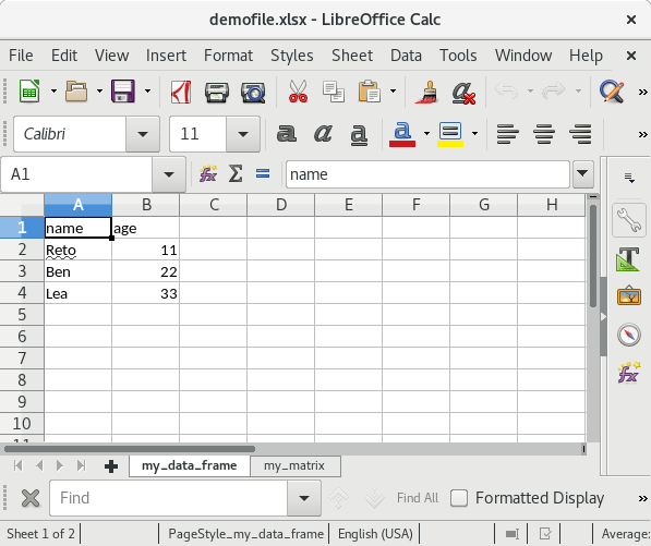
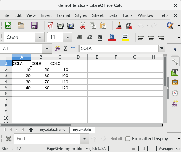
# Generate two objects
# A simple data.frame
my_df  <- data.frame(name = c("Reto", "Ben", "Lea"),
                     age  = c(11, 22, 33))
# And a small matrix
my_mat <- matrix(1:12 * 10, nrow = 4,
                 dimnames = list(NULL, c("COLA", "COLB", "COLC")))
We now write the two objects into one XLSX file. The first argument
to write.xlsx() (openxlsx)
is either a single object or a list of objects. In case of a list,
a new XLS sheet will be created for each object. If the list
is named, the names will be used to name the sheets.
library("openxlsx")
write.xlsx(list("my_data_frame" = my_df, "my_matrix" = my_mat),
           file = "testfile_write.xlsx")
If you open this file in Excel (screenshots are from OpenOffice) the content of the XLSX file should look as follows:
Summary
Yes, XLS/XLSX files can, of course, be handled by R. However, it most often makes things more difficult and not easier.
Thus the suggestion is to avoid spreadsheets to store/load data if possible. CSV files are a convenient alternative and can be read by most programming languages without the requirement of having additional packages/modules installed.
12.6 Additional functions
There are other ways to read text files. To mention two: readLines()
reads a text file line-by-line, scan() reads all elements stored in a
text file and tries to convert it into a vector.
Note that this is not an essential part of this course and we will (quite likely) never use it, however, feel free to read trough this section.
Read file line-by-line
The function readLines() is reading a file line-by-line.
Usage
Important arguments
con: a connection object or, in the simplest case, a character string (file name)n: maximum number of lines to read (n = -1means “all”)encoding: the encoding is getting important if the files you would like to read uses an encoding different from your system encoding.
Note: readLines() can also be used for user-interaction using con = stdin() (default). Try to run the following lines of code and see what happens!
For demonstration purposes I have downloaded the latest 1000 tweets from Donald Trump (rtweet) and stored the user ID, time created, and the content of the tweet in a simple ASCII file (download file). Each line contains one tweet.
Let’s read this file:
# Reading the first two lines only
content <- readLines("data/donald.txt")
c(class = class(content), length = length(content))
## class length
## "character" "1000"readLines() returns us a character vector with the same length as we have
lines in the file - in this case 1000. Let’s check the first two elements
of the vector content (first 80 characters only, see ?substr):
## [1] "25073877 - 2019-10-01 13:19:24 - ....the Whistleblower, and also the person who "
## [2] "25073877 - 2019-10-01 13:19:23 - So if the so-called “Whistleblower” has all sec"
Seems he had some problems with the whistleblower and the Ukraine affair in
October 2019. As you can see, readLines() does not care about the actual format
of the data, each line is simply read as one character string. As the tweets strongly
vary in their length, the length of these characters also strongly differs.
Just as a motivational example: what’s Donalds preferred time to tweet?
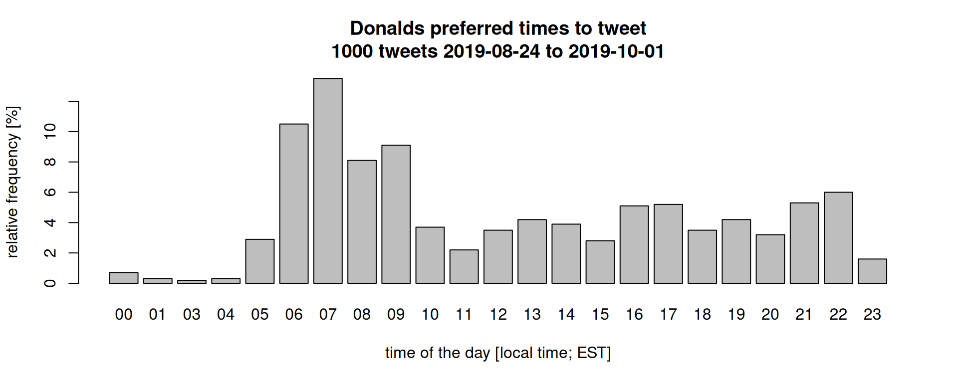
The R script for this plot can be downloaded here but uses some additional commands we have not discussed. We could also check how often he referenced himself (his twitter user or his name):
# Mentioned "realDonaldTrump" or "Trump" in general (in 1000 tweets)
c(realDonaldTrump = sum(unlist(gregexpr("realDonaldTrump", content, ignore.case = TRUE)) >= 0),
  Trump           = sum(unlist(gregexpr("Trump", content, ignore.case = TRUE)) >= 0))
## realDonaldTrump Trump
## 84 215We can also use readLines() to read other file formats as e.g., a website.
Let’s read the content of the entry page of the Universität Innsbruck
and try to find all links:
# Read the website
content <- readLines("https://uibk.ac.at", warn = FALSE)
c(class = class(content), length = length(content))
## class length
## "character" "641"# Try to find all links (href's)
hrefs <- unlist(regmatches(content, gregexpr("(?<=(href=\")).*?(?=\")", content, perl = TRUE)))
head(hrefs)## [1] "/static/uniweb/images/icons/favicon.a28011f62af2.ico"
## [2] "https://www.uibk.ac.at/de/"
## [3] "https://www.uibk.ac.at/de/"
## [4] "https://www.uibk.ac.at/de/"
## [5] "https://www.uibk.ac.at/en/"
## [6] "/static/uniweb/css/default.03715b74df98.css"Well, for parsing html/xml one should rather use an extra package (e.g.,.
xml2), but you can
also have fun with readLines()! :)
Writing lines works vice versa: we can use writeLines() to write a vector
into a file, each element of the vector will create one line in the file.
A small example:
# Create a vector to store in a file
names <- c("Reto", "Annika", "Peter", "Lea")
# Write the vector into a file
writeLines(names, "testfile.txt")
Once called, R creates the file "testfile.txt" on your disk which should now look
as follows:
Reto
Annika
Peter
Lea
CSV and Metadata
In one of the examples in the section Read custom CSV we have had an example where a CSV file contained some meta information in form of comments (the file “data/homstart-innsbruck-2.csv”).
What if we could write custom files with header information? Well,
the functions write.csv() and write.table() do not allow us to add
meta information in comment-form to a new file, but we can make use
of a combination of wirteLines() and write.table() to
create such files (write.csv() does not work as it has no append option).
Imagine the following situation: we have a data set data (a data.frame) with
some temperature and precipitation records:
data <- data.frame(month = c("Jan", "Feb", "Mar"),
                   year  = c(2019, 2019, 2019),
                   temperature = c(-1.3, 2.5, 4.9),
                   precipitation = c(0.0, 10.4, 15.3))
data
## month year temperature precipitation
## 1 Jan 2019 -1.3 0.0
## 2 Feb 2019 2.5 10.4
## 3 Mar 2019 4.9 15.3And a character vector with some meta information:
meta <- c("month: abbrevation of the month, engl format",
          "year: year of observation",
          "temperature: monthly mean temperature in degrees Celsius",
          "precipitation: monthly accumulated precipitation in mm/m2")
What we will do now is to:
- Write
meta: modify the strings (add"#";paste()does it for us) and write each entry of the character string into our output file, one line per element using the functionwriteLines() - Append the
datausingwrite.table()
Warning: writeLines() appends data to a file. If the file already exists,
it will simply add the new content at the end of the file. One way to prevent
this is to delete the file if it exists before we call writeLines().
There are other ways (e.g., use a file connection, see ?writeLines and ?open).
But let’s keep it “simple”:
# Name of our csv output file
outfile <- "tempfile_csv_with_meta.csv"
# If the output file exists: delete it
if (file.exists(outfile)) { file.remove(outfile) }
## [1] TRUE# Now write the meta information into the file
writeLines(paste("#", meta), con = outfile)
# Next, APPEND the data using write.table
write.table(data, file = outfile,
sep = ",", row.names = FALSE,
append = TRUE) # <- important!## Warning in write.table(data, file = outfile, sep = ",", row.names = FALSE, :
## appending column names to fileNote that write.table() gives us a warning as we use append = TRUE
but, at the same time, write the header (column names). As this is exactly
what we want to, we can ignore the warning.
Afterwards, the content of the file "tempfile_csv_with_meta.csv" should look as follows:
# month: abbrevation of the month, engl format
# year: year of observation
# temperature: monthly mean temperature in degrees Celsius
# precipitation: monthly accumulated precipitation in mm/m2
"month","year","temperature","precipitation"
"Jan",2019,-1.3,0
"Feb",2019,2.5,10.4
"Mar",2019,4.9,15.3
Scan
Usage
scan(file = "", what = double(), nmax = -1, n = -1, sep = "",
     quote = if(identical(sep, "\n")) "" else "'\"", dec = ".",
     skip = 0, nlines = 0, na.strings = "NA",
     flush = FALSE, fill = FALSE, strip.white = FALSE,
     quiet = FALSE, blank.lines.skip = TRUE, multi.line = TRUE,
     comment.char = "", allowEscapes = FALSE,
     fileEncoding = "", encoding = "unknown", text, skipNul = FALSE)
Important arguments
file: the name of the file to read data values from.what: the type of ‘what’ gives the type of data to be read. Supported are ‘logical’, ‘integer’, ‘numeric’, ‘complex’, ‘character’, ‘raw’, ‘list’.- A lot of arguments like in
read.table()such asn,sep,dec,skip,nlines,na.strings, … (see?scan).
The function scan() tries to extract all values of a specific type
from an unstructured text file. The file
scan_integer.txt
contains a series of integer values and missing values N/A.
3131 N/A  2866 8148 4483 4058 7286 2845 6840 7353 5011 2500 4432 2694 9688
8602 9064 1572 5361 4722 7833 8424 8897 6852 4453 5835 7860 7989 2243 2256

4686 2248 6524 N/A  7708 5852 5166 3642 7796 1757 1953 5849 3348 7839 3115
8168 N/A  5866 8382 5430 5698 5716 8703 6638 8205 4490 3051 6149 7586 1860

9342
5406 3143 7464 8574 N/A

8836 3861 8217 2781 9872 8445 9637 8210 8201
6357 7060 4840 7244 5257 2393 8809 6808 2621 6798 9375 2458 1183 6518 3456
We can try to extract all integers as follows:
## [1] 3131 NA 2866 8148 4483 4058## [1] "integer"This can sometimes be useful to read files which have been written as a stream (‘loosely’ added values).